 FEXLINK Research Institute
The short answer
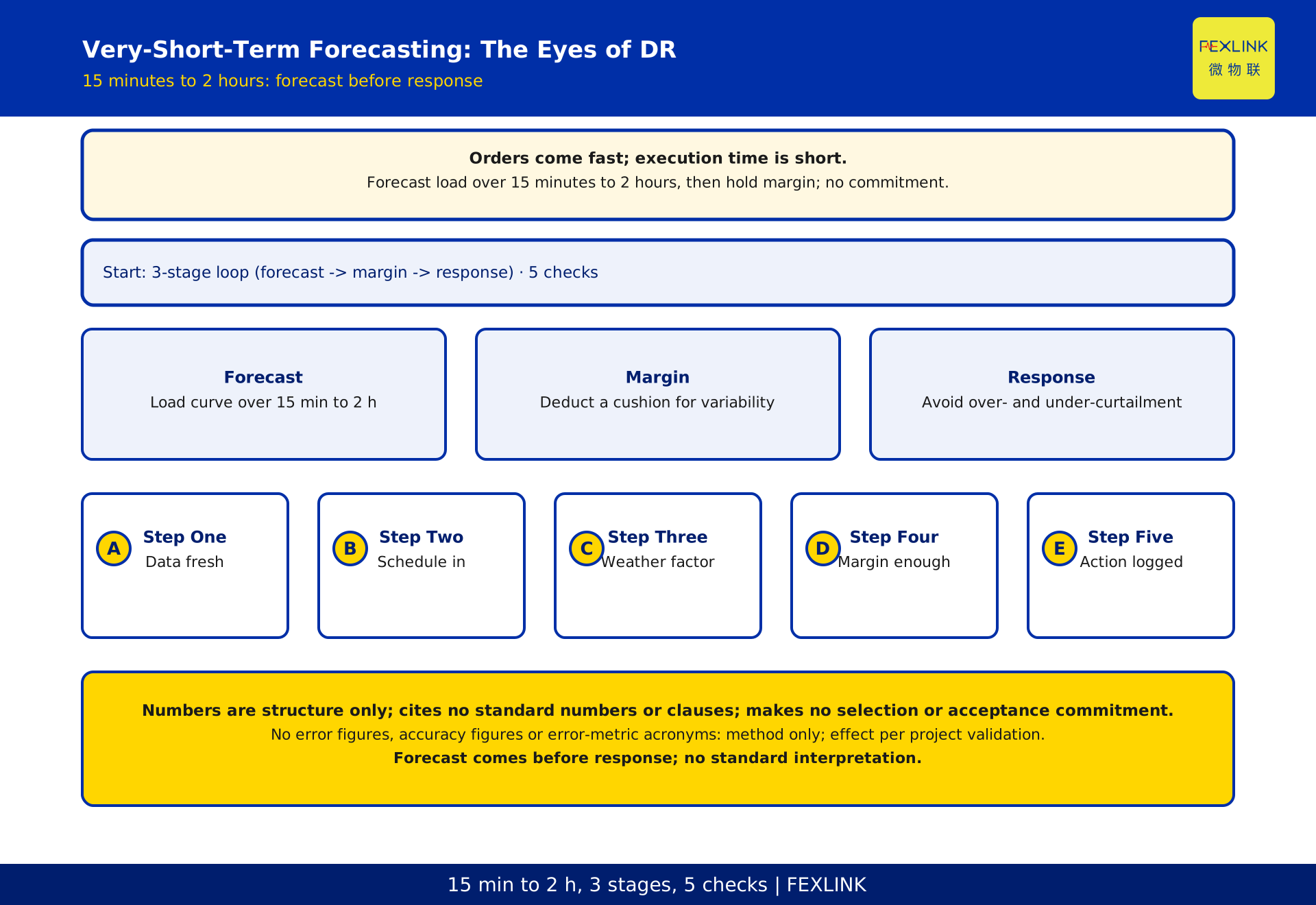
Demand response must anticipate the load curve for the next 15 minutes to 2 hours before the dispatch order arrives, so that flexible resources can be sized with the right reserve margin. That is why very-short-term load forecasting is called the eyes of demand response. Waiting for the order and then checking the meters usually ends in either over-curtailment that disrupts production or under-curtailment that loses revenue. Very-short-term forecasting uses time-series models combined with recent measurements and production schedules to work out roughly where the load will be, and then decides how much flexible headroom to keep. This article sets out the 3-stage forecast-to-margin-to-response loop and a 5-step check method. It does not cover how error metrics are scored; it cites no standard numbers or clauses and makes no conformance claims; it gives no accuracy, error percentages or effect figures, all subject to platform rules and project validation. It constitutes no selection or acceptance commitment.
Why response must forecast before acting
The response action happens after the order arrives, but the time left to execute is short. If you wait for the order to check the load, find resources and work out how much can be shifted, it is often too late — you either miss the response window or report a capacity by feel and end up over- or under-curtailing. Forecasting absorbs that delay in advance: before the order comes, you already know roughly where the load will sit over the next short interval and which direction it is moving, so you can judge which resources have spare capacity, how much, and whether moving them will disrupt production. The order must therefore be forecast first, margin second, response third — forecasting is the cause, holding margin is the link, and an accurate response is the result. Reversing that order is reporting capacity with your eyes shut. The core increment here is exactly this forecast-to-margin-to-response loop; how error metrics are scored belongs to a separate article and is not developed here.
Why the 15-minute to 2-hour scale is special
The very-short-term window runs from 15 minutes to 2 hours, and this scale is distinctive. It is far shorter than day-ahead forecasting, which need not answer tomorrow's total consumption; it is a little longer than real-time control, and just covers the preparation window from receiving the order to breaking it down and completing execution. A longer window means little to site dispatch, while a shorter one leaves no time to arrange resources. Landing in the 15-minute to 2-hour band means the forecast can directly decide how much flexible margin to hold right now: the near end keeps recent measurements fresh and credible, and the far end is close enough that the production schedule stays fairly stable. Understanding this scale explains why very-short-term forecasting cannot simply copy day-ahead methods nor force real-time control thinking — it is tailored to the response preparation window.
Main methods: time-series models and gradient boosting
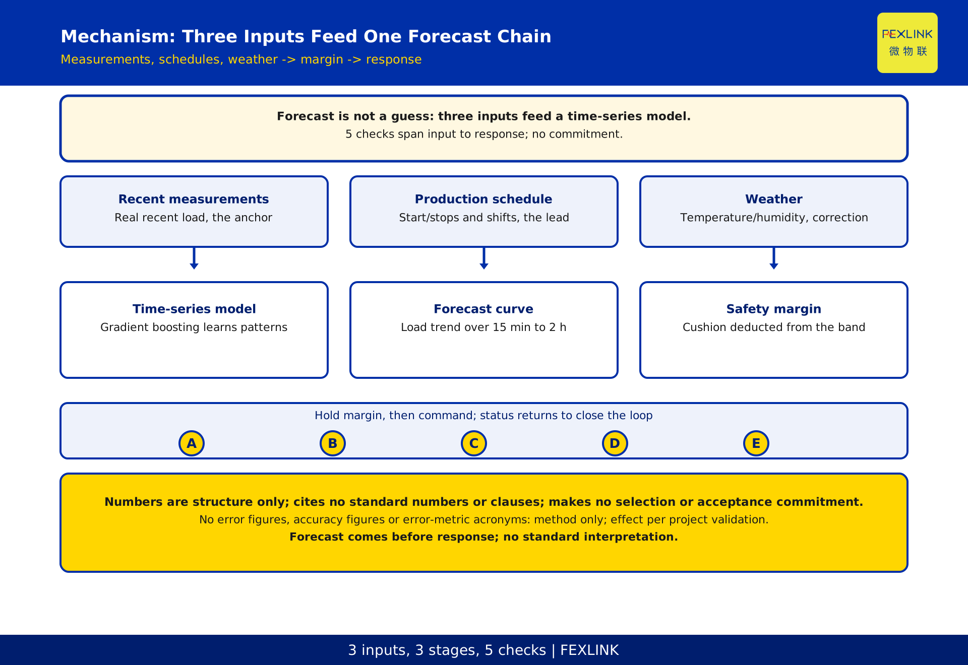
Very-short-term forecasting relies mainly on time-series models, among which gradient boosting methods are widely used. The idea is not mysterious: feed past load curves, recent measurements, production schedules and weather into the model, let it learn from history how the load usually behaves under such input combinations, then apply that pattern to the current inputs to output a forecast curve for the near future. Why gradient boosting rather than others? Because it handles tabular data, non-linear relationships and feature combinations well, and can give usable forecasts without fully modelling the physical process. One boundary must be clear: this article is about how forecasting supports response, not algorithm comparison or an accuracy contest — which model to use, to what precision and at what accuracy belong to methods and metrics, outside this scope. The model may even be a black box; what matters is how its forecast curve becomes response margin.
Three input types: recent measurements, production schedules, weather
Forecast quality depends heavily on the data fed in. Very-short-term forecasting uses three main inputs. First, recent measurements — the real load and key-circuit data over the last interval, closest to the current state and the anchor of the forecast. Second, production schedules — workshop start/stops, shift arrangements, planned maintenance; these determine where the load is likely to head and carry information people know before the curve shows it. Third, weather — temperature, humidity and other external factors that affect cooling and process loads, used as a corrective input. Of the three, recent measurements are the base, schedules the lead, weather the correction. Without recent measurements the forecast drifts; without schedules it cannot see production changes; without weather data a sudden shift throws it off. The ESX smart edge computing gateway plays its part right here on the data side: it collects recent measurements and key-circuit data under a unified clock, giving the forecast a fresh anchor; the specific connection follows project circuit and metering requirements, not developed here.
Turning forecast error into response margin
A forecast is never perfectly accurate; error always exists. The point is not to eliminate error but to translate it safely into response margin. The method is this: the forecast curve gives a central estimate, and a band — roughly the range the load will most likely fall in — is derived from recent variability. When reporting flexible capacity, you do not take the central estimate at face value; you deduct a safety cushion from it, and that cushion is the margin. The wider the band and the larger the fluctuation, the thicker the cushion, and the more conservative the reported capacity. Even if the forecast is off, the deviation is absorbed by the margin instead of becoming over- or under-curtailment. Here we describe only the method action of converting error into margin, giving no error percentages or accuracy figures — those metrics and their scoring belong to a separate article. The one thing operators should remember is this: a forecast value cannot be reported as a commitment; a layer of margin must sit in between.
The chain from forecast to command
String the steps together and you get a complete execution chain: the model outputs a load curve for the next 15 minutes to 2 hours; the operator judges how much can be shifted and how much margin to keep against the flexible-resource list; a command goes to the execution end, which acts and returns its status; finally the measured data checks back whether the response met expectations. In this chain, forecast is the start, margin the buffer, command the action, and return-and-check the closed loop. Miss any link and the response degrades: no forecast is blind reporting, no margin is recklessness, no status return means you cannot confirm the action happened. The value of understanding this chain is that when a response misses target, you can trace segment by segment — was the forecast off, the margin too thin, the command not delivered, or the execution end unmoved — instead of blaming it all on a bad forecast. This article gives the tracing framework, not the parameters of each segment.
The ESX role on the data side
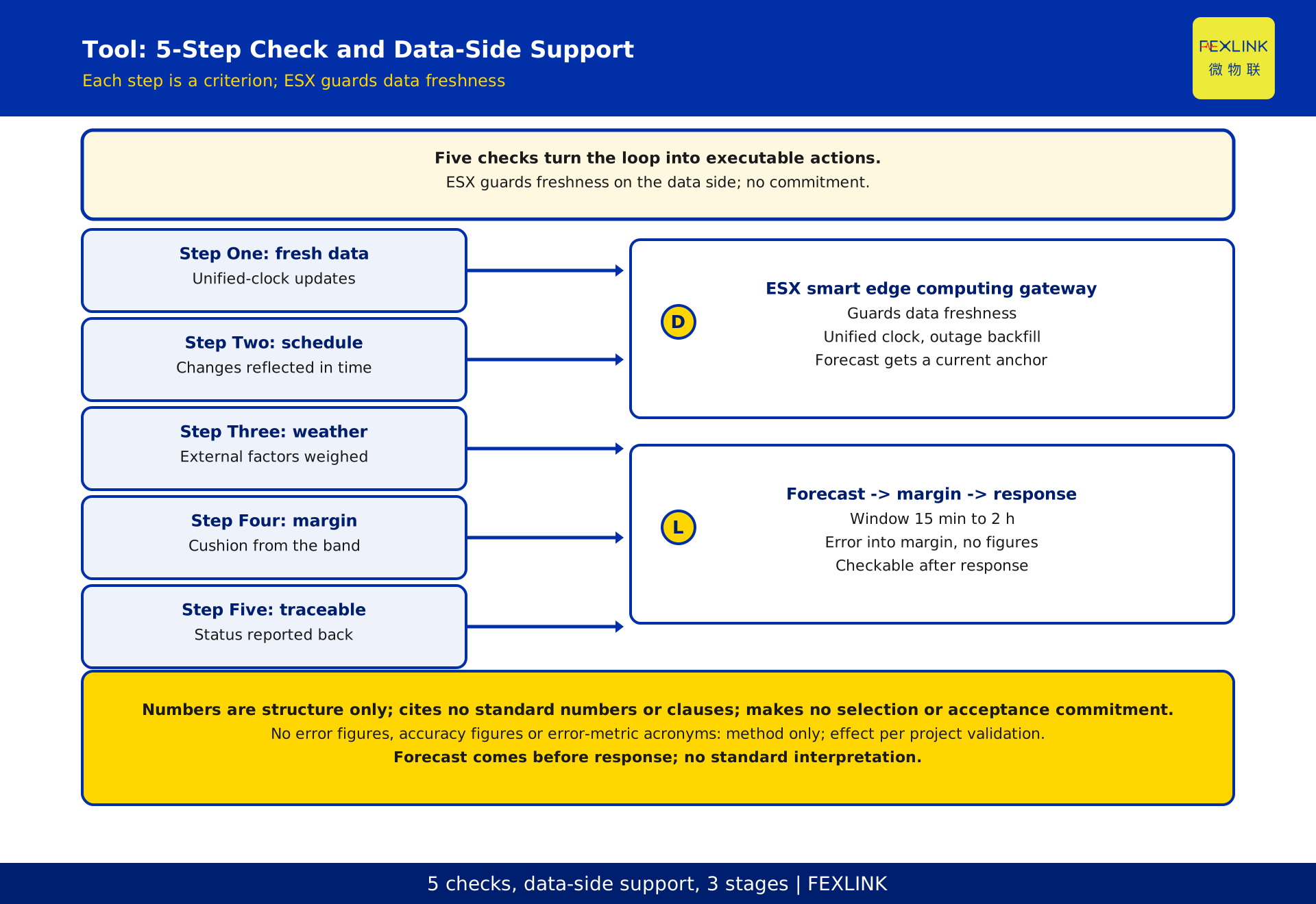
Back to the input-data link. Very-short-term forecasting fears stale data most — a few minutes of lag in the measurements and the forecast already diverges from the current state. The role the ESX smart edge computing gateway carries on the data side is to guard that freshness: it collects key circuits and recent load under a unified clock so the model gets data as close to the present as possible, and on network loss it backfills first and completes after recovery, avoiding a data gap that would leave the forecast without an anchor. To be clear, ESX is the execution end of the data chain — it delivers raw data promptly, completely and on a common clock to the forecasting stage; it does not do the forecasting itself, nor decide how much margin to keep. Concrete models, interfaces and access follow the latest selection manual and project design files; this article constitutes no selection or acceptance commitment.
Common issues in deployment
Three issues come up most often in deployment. First, data lag: measurements enter the system slowly, the model sees the past, and the forecast drifts — the fix is to check the collection chain and the clock. Second, schedule changes: a plan is adjusted at short notice while the model still computes on the old schedule, and the forecast cannot keep up — the fix is to feed schedule updates into the inputs in time. Third, sudden weather shifts: temperature or cloud cover changes sharply beyond the range covered by history — the fix is to keep weather as an input and tighten the margin when shifts occur. These three map to the weak points of the three input types, and a check along data, schedule and weather is enough to locate the cause. These are work-level verification methods, not accuracy promises; actual forecasting performance depends jointly on data quality, the model and site conditions, and must be confirmed by qualified personnel against project documents.
The five-step check method
Distil the whole logic into an executable five-step check. Step one, confirm recent measurements are updating under a unified clock and the data is fresh. Step two, confirm the production schedule is in the inputs and changes are reflected in time. Step three, confirm weather and other external factors are considered as corrections. Step four, confirm the forecast output has deducted a safety cushion against the error band and the margin is enough. Step five, confirm the chain is complete, action status is reportable, and the response can be checked afterwards. The five steps correspond to the five key points — the forecasting premise, the time scale, the method, the inputs, and error-to-margin — and checking them one by one locates which link has the problem. Each step gives a judgement criterion rather than a parameter value: is the data fresh, is the schedule included, is the margin enough, is the action traceable — all checkable on site without relying on any single figure. The value of this list is turning forecasting-supports-response from a phrase into executable actions.
FAQ
Q: What exactly does very-short-term load forecasting predict?
A: It predicts the load curve for the next 15 minutes to 2 hours — not tomorrow's total consumption, but roughly where the load will sit and which way it is moving over this short preparation window. Its goal is concrete: tell the operator how much flexible margin to keep.
Q: Why not wait for the order and then work out how much can be shifted?
A: Because the time left to execute is short; checking the load, finding resources and sizing capacity on the spot is often too late, ending in over-curtailment that disrupts production or under-curtailment that loses revenue. Forecast first, keep margin second, respond third — that absorbs the delay.
Q: Is gradient boosting mandatory?
A: It is a widely used class of time-series model for very-short-term forecasting and handles tabular data and non-linear relationships well, but it is not the only choice. This article is about how forecasting supports response, not algorithm comparison or an accuracy contest; which model to use depends on project conditions.
Q: Can forecast error cause a response to miss target?
A: It can pose a risk, but margin can absorb it. The approach is not to report the forecast at face value but to deduct a safety cushion against recent variability — the wider the band, the thicker the cushion. This article describes only that conversion method, giving no error percentages or accuracy figures.
Q: How does this differ from articles on error metrics?
A: This article covers why very-short-term forecasting is a response prerequisite, its time scale, methods, inputs and how error becomes margin, landing on the forecast-to-margin-to-response loop. How error metrics are defined and scored is a separate topic not developed here.
Scope and limitations
This article addresses energy managers and demand-response operators, setting out why very-short-term load forecasting is a prerequisite for demand response and the forecast-to-margin-to-response loop with a five-step check method. It does not cover how error metrics are scored, algorithm comparison or accuracy contests, or the full system of day-ahead and short-term forecasting. It cites no standard numbers or clauses and makes no conformance claims; it gives no accuracy, error percentages or effect figures, all subject to platform rules and project validation. This article constitutes no selection or acceptance commitment and no standard interpretation; the generator does not self-approve, and publication requires independent verification; implementation is carried out by licensed electrical and professional personnel under site procedures, and this article replaces neither electrical design nor site safety rules. Actual forecasting performance depends jointly on data quality, the model and site conditions, and must be confirmed by qualified personnel against project documents.
Frequently Asked Questions
What exactly does very-short-term load forecasting predict?
It predicts the load curve for the next 15 minutes to 2 hours — not tomorrow's total consumption, but roughly where the load will sit and which way it is moving over this short preparation window. Its goal is concrete: tell the operator how much flexible margin to keep.
Why not wait for the order and then work out how much can be shifted?
Because the time left to execute is short; checking the load, finding resources and sizing capacity on the spot is often too late, ending in over-curtailment that disrupts production or under-curtailment that loses revenue. Forecast first, keep margin second, respond third — that absorbs the delay.
Is gradient boosting mandatory?
It is a widely used class of time-series model for very-short-term forecasting and handles tabular data and non-linear relationships well, but it is not the only choice. This article is about how forecasting supports response, not algorithm comparison or an accuracy contest; which model to use depends on project conditions.
Can forecast error cause a response to miss target?
It can pose a risk, but margin can absorb it. The approach is not to report the forecast at face value but to deduct a safety cushion against recent variability — the wider the band, the thicker the cushion. This article describes only that conversion method, giving no error percentages or accuracy figures.
How does this differ from articles on error metrics?
This article covers why very-short-term forecasting is a response prerequisite, its time scale, methods, inputs and how error becomes margin, landing on the forecast-to-margin-to-response loop. How error metrics are defined and scored is a separate topic not developed here.