 FEXLINK Research Institute
The short answer
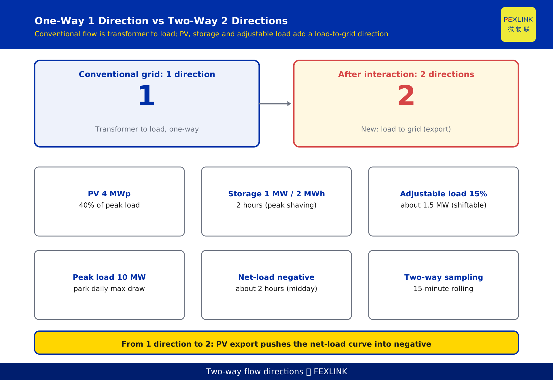
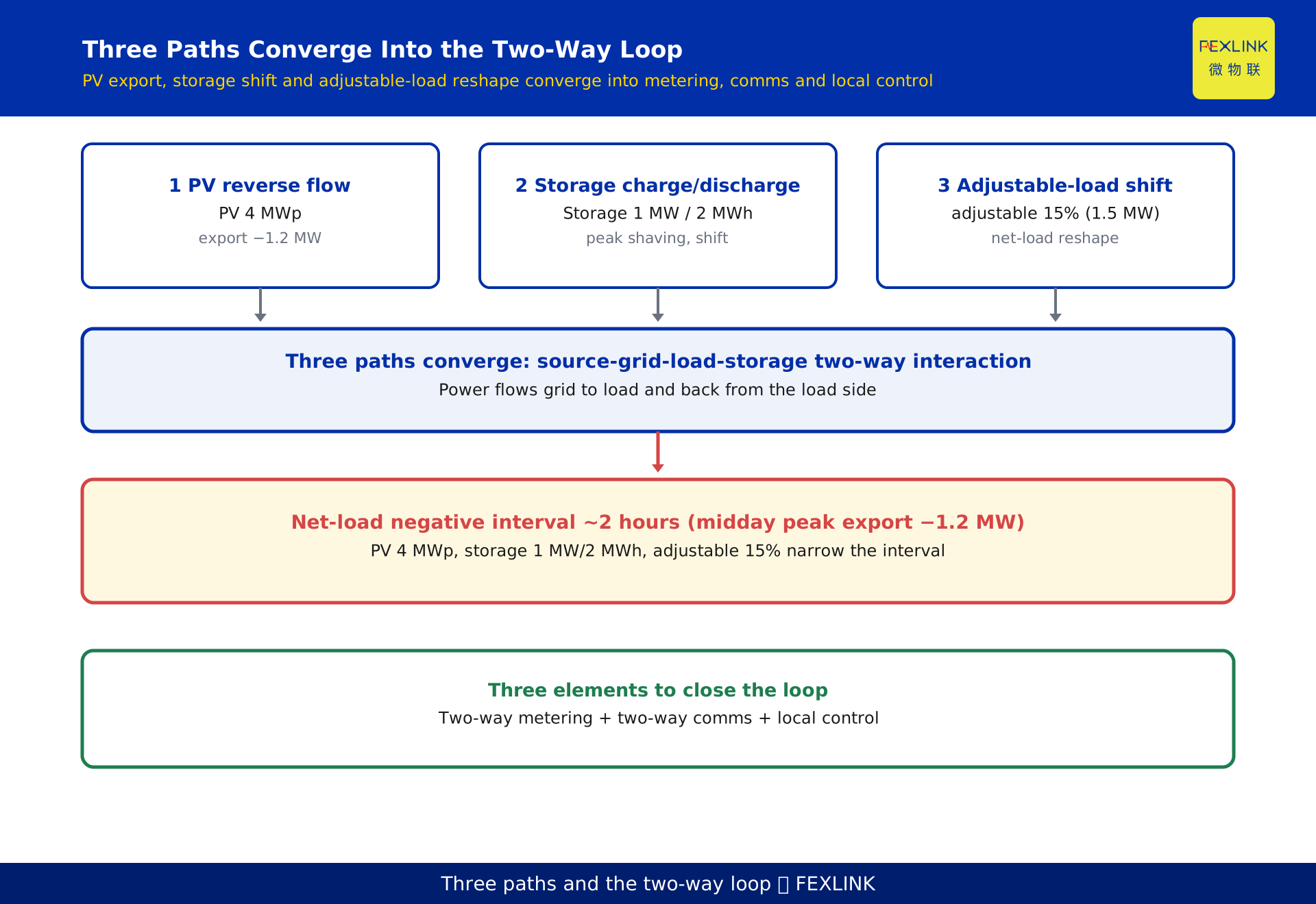
In a conventional distribution network the power flow is one-way: active power moves from the grid, through the distribution transformer, down to the load — a single fixed direction. Once distributed photovoltaic (PV), storage, and adjustable load are added, that direction is no longer fixed. When PV output exceeds local load, power flows backward to the transformer and even to the main grid (reverse power flow). A battery stores energy by absorbing power when charging and delivers it when discharging. Adjustable load shifts consumption from peak to off-peak hours. The system therefore needs both two-way metering (recording forward and reverse energy) and two-way control (able to act on the source and the load alike) to close the interaction loop. The rest of this article breaks that process down.
1. What "power flow" actually means
In power systems, "power flow" means the direction and magnitude of active power moving through the grid. The "how much electricity was used" we talk about every day is essentially the portion of power absorbed by the load at the end of the flow. In the traditional analysis model, the distribution transformer is a natural boundary: power enters on the high-voltage side and leaves on the low-voltage side, moving top-down.
The first step to understanding two-way interaction is to pull "direction" out of the defaults. Power flow is not an abstraction; at every moment it has a definite direction. When that direction changes, everything the system has to handle changes with it.
2. Why conventional networks are one-way
A classic radial distribution network places the source at the substation side and the load at the far end. Power leaves the 110 kV / 10 kV substation, travels through the distribution transformer, and reaches the customer — in a fixed direction. On every segment of the feeder, active power flows from the busbar to the load; no local source feeds power back.
This is a "source-follows-load" one-way model: dispatch only cares "how much does the load want, how much should the source supply", the grid side is always the supplier, and the customer side is always the consumer. The corresponding metering only needs to record one direction — how much the customer drew from the grid. This model ran for over a century: simple, reliable, but with one hidden assumption — no power is produced locally.
3. PV flips the direction
Distributed PV is installed on the load side — rooftops, carports, idle roof areas. When daylight is strong and local load is small, local generation exceeds local consumption, and the surplus flows back along the feeder to the transformer and even reverses into the main grid. This is "reverse power flow".
Reverse flow brings two tangible electrical consequences. First, feeder node voltage is pushed up: with a source injecting at the end, the direction of the voltage drop reverses, and end-of-line voltage can be driven close to its upper limit. Second, the transformer may see reverse power, while conventional one-way metering only records "customer draw" — energy sent back is either missed or wrongly counted as consumption.
Technical fact: after distributed PV is grid-connected, when local output exceeds local load, the feeder exhibits reverse power flow and end-of-line node voltage may rise — a well-known point in distribution grid interconnection analysis (public distribution-grid references; grid-tied inverter principles).
Using the worked park example constructed in this article: the park's peak load is 10 MW, rooftop PV is 4 MWp, so PV is 40% of peak. At midday the load dips to a 2.4 MW trough while PV peaks at 3.6 MW output; net load = 2.4 − 3.6 = −1.2 MW, i.e. 1.2 MW is exported backward, for a negative interval of about 2 hours. In other words, on the same day this park is "supplied by the grid" in the morning and evening, but for those 2 midday hours it is "supplying the grid".
4. How storage flattens the load curve
Storage can be seen as a "load that can reverse": charging, it is a load (absorbing power); discharging, it is a source (delivering power). Scheduling discharge into the load peak and charging into the load trough and the PV-rich period shifts and flattens the net-load curve — peaks are shaved, troughs are filled.
Continuing the example: the park has 1 MW / 2 MWh (2-hour) storage. At the evening peak it discharges 1 MW, displacing part of the power that would otherwise be drawn from the grid; at midday, when PV is strong and load is low, it charges and absorbs 1 MW, consuming most of the 1.2 MW that would otherwise be exported. The result: the original −1.2 MW export is pushed down, the negative interval shortens, and the evening purchase peak also drops.
The key here is "time shifting": storage does not change total consumption, only when in the day it occurs, bringing the net-load curve closer to a flat line.
5. How adjustable load reshapes the net load
Adjustable load means load that can be interrupted or shifted — central air conditioning, storage-type heat pumps, production lines that can be delayed. It adds no equipment; it only changes "when to consume".
Moving part of the peak-period consumption into the PV-rich or low-load period directly cuts the net-load peak and narrows the negative interval. In the example, the park's adjustable load is about 1.5 MW (15% of peak); shifting this 1.5 MW from the evening peak to the midday PV window both lowers the evening purchase peak and absorbs part of the midday export.
Storage is "store"; adjustable load is "move" — different mechanisms, same goal: smoothing the net-load curve and reducing the two-way impact on the grid.
6. Stacking the three on one net-load chart
Net load = load − distributed-source output. Overlay the three lines and it is clear: the raw load curve peaks in the evening, the PV output curve peaks at noon, and subtracting them gives the net-load curve — dipping into a negative interval at noon while still carrying an evening peak.
Storage and adjustable load are exactly what flatten this net-load curve. Storage shaves the evening peak and fills the midday trough; adjustable load moves evening-peak consumption to midday. Once the three work together, the net-load peak falls and the negative interval narrows — the system moves from "one-way draw only" to "controllable in both directions".
This chart also explains why PV alone is not enough: PV only creates the negative interval; it is storage and adjustable load that flatten both the negative interval and the peak.
7. Why two-way metering and communication are mandatory
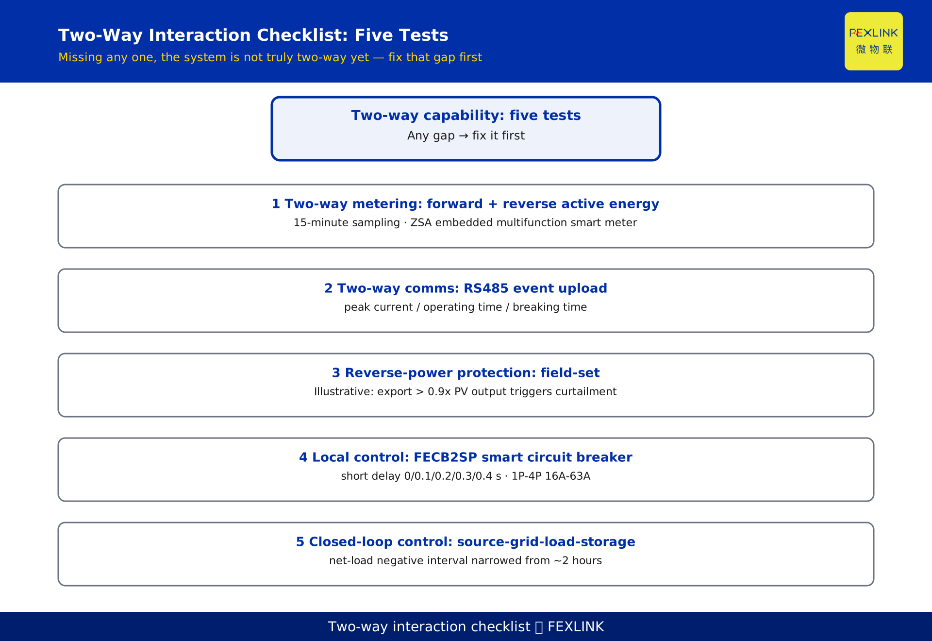
When power can flow both ways, one-way metering falls short. You must record separately the energy the customer draws from the grid (forward) and the energy sent back (reverse); otherwise billing, subsidy settlement, and line-loss accounting all go wrong — exported energy must not be quietly dropped or counted as consumption. This is "two-way metering".
Paired with it is "two-way communication": the meter does not just show a local number; it must upload forward/reverse data and key events (e.g. reverse-power limit breach, short circuit) to the platform so the system can run closed-loop control. Mechanically, the net-load curve must be captured at a 15-minute rolling interval to reliably catch the about 2-hour negative interval at midday and the evening peak.
At the metering layer, the ZSA embedded multifunction smart meter sits in the metering tier of the "metering–monitoring–control" three-tier structure, handling the metering settlement of "how much energy was used and how the bill is calculated"; some versions carry 4DI/2DO and can record both forward and reverse active energy, providing the underlying data for two-way metering.
8. Two-way control must land on executable devices
Measuring is not enough; you must be able to "act". Two-way control needs locally controllable actuators: when strong PV drives a reverse-power limit breach, you need a switch that can open/close quickly and upload event data; when load must be shifted, you need circuit breakers that can be switched on schedule.
The FECB2SP smart circuit breaker has adjustable short-time delay (0 / 0.1 / 0.2 / 0.3 / 0.4 s), covers 1P/2P 16A/32A AC230V and 3P/4P 32A/63A AC400V, carries RS485, and can upload the peak current, operating time, and breaking time of a short-circuit event to the platform — providing the handle for local control and event traceability.
A note: where reverse-power protection settings, voltage-limit thresholds, or switching times are mentioned, they are illustrative or methodological only; concrete values are subject to field design. This article gives no fixed code values and cites no specific standard clause numbers.
9. A worked example: one park
The numbers used above are summarized into one reproducible constructed example (declaration: the following figures are constructed to illustrate the mechanism and represent no real customer or project):
- Incomer at 10 kV with 2×1250 kVA transformers; park peak load 10 MW.
- Rooftop distributed PV 4 MWp, 40% of peak load.
- Storage 1 MW / 2 MWh (2 hours).
- Adjustable load about 1.5 MW, 15% of peak.
- Two-way acquisition at 15-minute interval.
- Midday: load trough 2.4 MW, PV peak output 3.6 MW, net load −1.2 MW, negative interval about 2 hours.
The conclusion is direct: with PV alone, the park shows a 2-hour, 1.2 MW export at midday and still an evening purchase peak; adding storage charging absorption and adjustable-load shifting narrows the negative interval and lowers the evening peak, turning the system from "one-way draw" into "two-way interaction".
10. FAQ
Q: Does installing PV automatically cause reverse flow?
Not necessarily. Reverse flow only occurs when local PV output exceeds local load, typically during midday low-load, strong-sunlight periods. On a cloudy evening with high load and little PV, flow stays conventional and one-way. How often reverse flow happens depends on PV penetration (PV capacity ÷ peak load) and the shape of the load curve.
Q: What is bad about reverse flow, and why manage it?
Reverse flow injects backward along the feeder and raises end-of-line node voltage, possibly pushing it above the upper limit; it also reverses transformer power, and one-way metering misses or miscounts the exported energy. The usual practice is reverse-power protection to limit export, or storage for local absorption. Concrete thresholds are subject to field design.
Q: How do storage and adjustable load differ?
Storage is equipment that moves power in time through charge/discharge, shaving both peak and trough. Adjustable load adds no equipment; it only changes when consumption happens, moving peak use to the trough or PV-rich period. Both smooth the net-load curve but by different mechanisms: one stores, one moves.
Q: How does two-way metering differ from a normal meter?
A normal meter records one direction (customer draw). Two-way metering must record forward (draw) and reverse (export) active energy separately; otherwise exported energy is either missed or counted as draw. For sites with PV and storage, two-way metering is the prerequisite for billing and line-loss accounting.
Q: How do I judge whether a park should adopt two-way interaction?
One criterion: first look at PV penetration — if PV capacity ÷ peak load exceeds roughly 15%–20%, you should assess reverse-power and voltage-limit risk and put two-way metering, two-way communication, and local control into the design; if penetration is low and load is stable, start with solid one-way metering and monitoring. Concrete thresholds are subject to field design.
Scope and limitations
- The flow direction, reverse flow, net-load curve, two-way metering, and two-way control discussed here are a mechanism review of distribution-network operation, applicable to medium- and low-voltage distribution networks integrating distributed PV, storage, and adjustable load.
- The figures for "a certain park" — PV 4 MWp, storage 1 MW/2 MWh, adjustable load 15%, peak 10 MW, midday net load −1.2 MW, negative interval 2 hours — are constructed examples to illustrate the mechanism and represent no real customer or project; actual projects must be calculated from site survey and measured data.
- Where reverse-power protection settings, voltage-limit thresholds, or switching times are mentioned, they are illustrative or methodological only and subject to field design; this article gives no fixed code values and cites no specific standard clause numbers.
- The specific model parameters of the ZSA embedded multifunction smart meter and the FECB2SP smart circuit breaker (short-time delay steps, current ratings, 4DI/2DO, RS485) are subject to the latest selection manual and product knowledge base; this article is not a selection or procurement recommendation.
- Two-way interaction retrofit involves grid connection and protection coordination and must be designed and built by qualified units per current codes; this article is mechanism education only and not an engineering instruction.
Frequently Asked Questions
From One-Way to Two-Way Power Flow
In a conventional distribution network the power flow is one-way: active power moves from the grid, through the distribution transformer