 FEXLINK Research Institute
The short answer
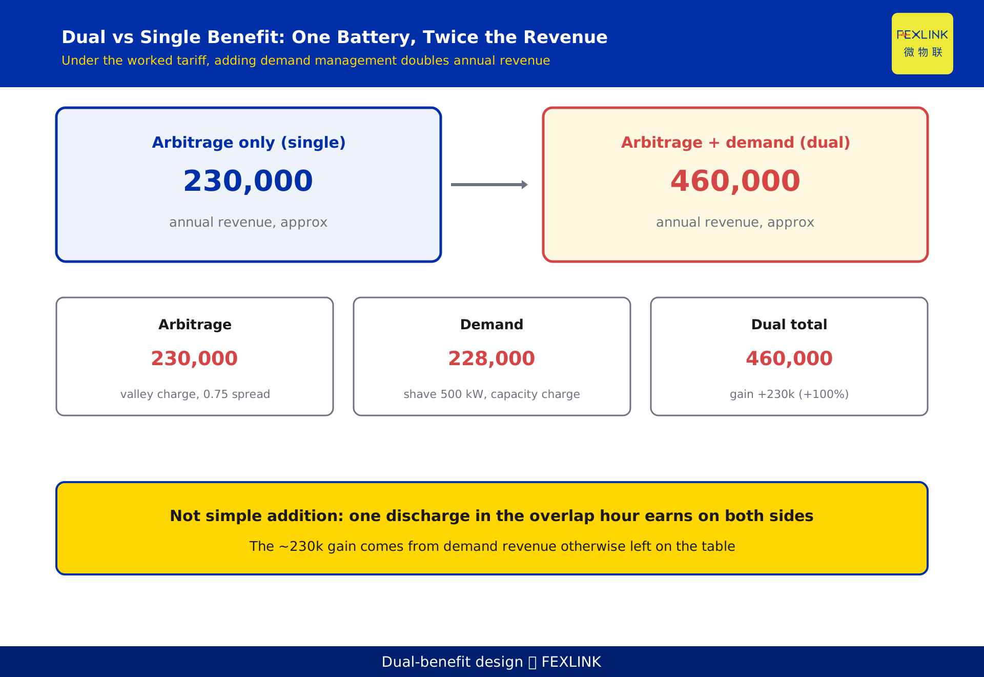
A factory's bill is squeezed from two sides: the peak-valley price spread and the demand (capacity) charge. One storage system can earn on both — as long as you stop letting it do only one job. The dual-benefit design stacks two strategies on the same battery: charge in the valley and discharge in the peak for arbitrage, and discharge again during the demand spike to shave the monthly peak and cut the capacity charge. The hard part is the energy management system (EMS) dynamically trading off the two goals under one shared SOC and power constraint, so arbitrage does not drain the battery before the shaving window arrives. In the worked example, the dual-benefit design yields about 460,000 yuan per year — double the roughly 230,000 yuan from arbitrage alone.
1. Where the two revenues come from
Most large industrial users pay a two-part tariff. The first part is energy charge, billed on kilowatt-hours consumed. The second is the basic (demand) charge, billed on transformer capacity or the monthly peak demand in kilowatts. Peak-valley arbitrage earns from the first part: buy low in the valley, sell (displace) high in the peak, keep the spread. Demand management earns from the second part: during the demand spike, discharge the battery to displace grid power, pull the monthly peak down, and the capacity charge falls with it.
The two targets are not the same. Arbitrage wants to cycle often and capture the spread on every kilowatt-hour. Demand management only cares whether those few peak-demand hours of the year got shaved; it can stay idle otherwise. One wants to use the battery hard; the other wants it ready for the critical moment — exactly where a single battery doing both tends to break unless scheduled deliberately. (Public information: China's large industrial users face a two-part tariff with time-of-use pricing, peak about 2–3 times valley.)
2. Why one battery can earn on both
The good news is that the high-value moments overlap. Arbitrage discharges in the peak window, and the factory's peak-demand spike usually lands in the same block of hours — morning production at full tilt, afternoon equipment all on, evening overtime. Those are both the most expensive hours and the hours most likely to set the monthly peak.
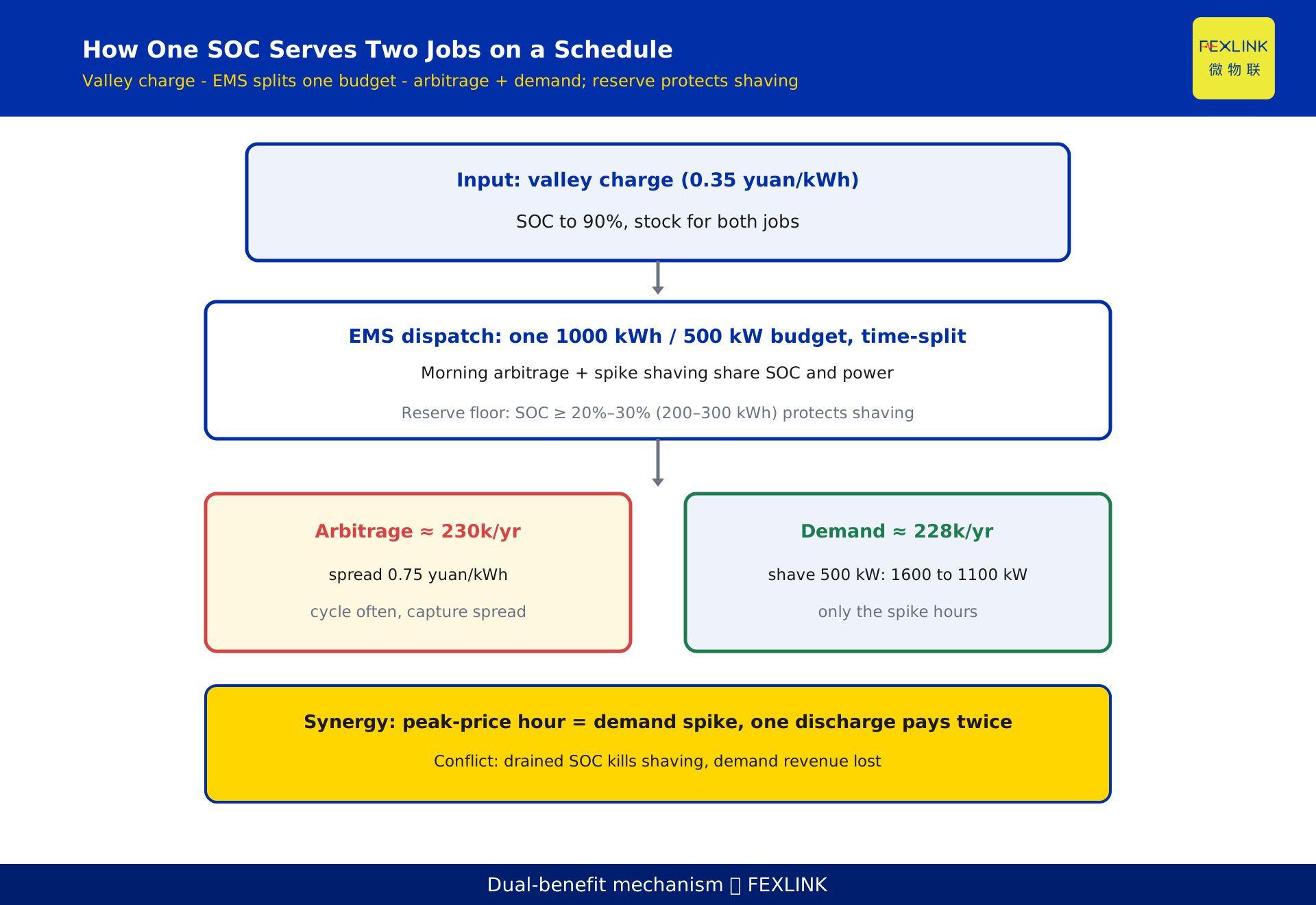
So a single discharge in such an hour earns the peak-valley spread (arbitrage) and lowers that hour's demand (demand management). One discharge, two payoffs: the "synergy dividend" of the dual-benefit design. In the example, a 1,000 kWh / 500 kW battery discharging 500 kW at the 1.10 yuan/kWh peak can pull the peak demand from 1,600 kW down to 1,100 kW in a single spike hour, saving about 228,000 yuan per year on the capacity charge alone.
3. How one battery takes both jobs on a schedule
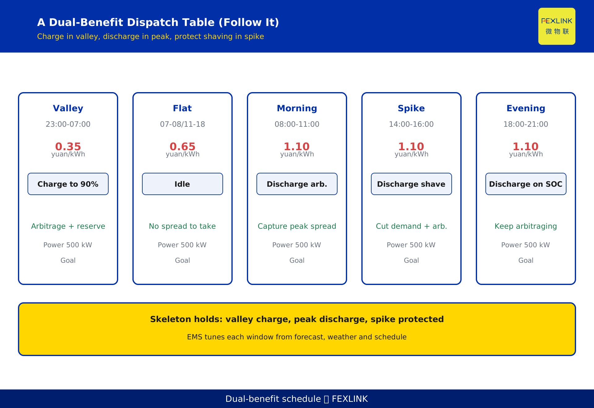
Because the synergy sits in the overlapping high-price, high-load window, the core of the design is a time-of-use task table that assigns the same SOC to different tasks in different windows:
- Valley (23:00–07:00, 0.35 yuan/kWh): charge hard, push SOC to a high level (about 90%). This stocks both the next day's arbitrage and the energy reserved for possible shaving.
- Flat (0.65 yuan/kWh): idle, neither charge nor discharge, because there is no spread to capture.
- Morning peak (08:00–11:00, 1.10 yuan/kWh): discharge for arbitrage, displacing peak grid purchases.
- Spike / demand window (14:00–16:00, 1.10 yuan/kWh): discharge to shave the peak and still capture the peak spread.
- Evening peak (18:00–21:00, 1.10 yuan/kWh): discharge on remaining SOC to keep arbitraging.
The key point: the morning arbitrage discharge and the spike shaving discharge draw on the same cells and the same SOC budget. They are not two parallel jobs; they are a sequential split of one capacity.
4. Splitting SOC and power: the reserve-threshold method
Conflict appears when the SOC budget is too thin to share. If the morning peak drains the battery for arbitrage, then by the time the real annual demand spike arrives in the afternoon the battery is empty, shaving capability is zero, and the most valuable capacity-charge saving of the year is lost.
The engineering fix is the "reserve-threshold method." The EMS first predicts when the day's peak demand will likely occur and reserves a minimum SOC floor for shaving (for example, keep SOC no lower than 20%–30%, roughly 200–300 kWh, enough to support 500 kW for 0.5–1 hour). Only the remaining energy is released to the arbitrage cycle. Power is allocated the same way: the 500 kW rated power is committed to shaving first during the spike, and any surplus serves the morning arbitrage. Both goals then fit inside one constraint without crowding each other out.
5. Finding and forecasting the demand spike
To shave demand you must first know where the "peak" is. The demand charge is usually billed on the month's maximum 15-minute average power, or a similar sliding window — so the real spike is not an instantaneous current but a load plateau sustained for ten-plus minutes. Identification takes three steps.
First, pull the last 12 months of hourly load curves and locate each month's peak demand — when and how large (in the example plant the original peak was about 1,600 kW, concentrated in 14:00–16:00). Second, separate "regular spikes" from "occasional spikes" — a regular one (every afternoon, all equipment on) is worth shaving daily with storage; an occasional one (a one-off trial run) needs its own economics. Third, align the spike hour with the peak-price window: the higher the overlap, the more a single discharge pays on both sides.
Forecasting relies on the EMS day-ahead load prediction: how much to charge and how much SOC to hold depends on tomorrow's spike. More accurate forecast, leaner reserve, larger arbitrage headroom.
6. A dual-benefit dispatch table you can put on the wall
Turning the logic above into a table yields an executable site dispatch schedule (parameters below are illustrative, not a real customer):
| Window | Price (yuan/kWh) | Battery action | Goal | Power |
|---|---|---|---|---|
| Valley 23:00–07:00 | 0.35 | Charge to 90% SOC | Stock arbitrage + reserve shaving | 500 kW charge |
| Flat 07–08 / 11–18 | 0.65 | Idle | — | 0 |
| Morning peak 08–11 | 1.10 | Discharge (arbitrage) | Arbitrage | 500 kW discharge |
| Spike demand 14–16 | 1.10 | Discharge (shave + arbitrage) | Cut demand + arbitrage | 500 kW discharge |
| Evening peak 18–21 | 1.10 | Discharge on SOC | Arbitrage | ≤500 kW |
This table is a tool, not a statute. In operation the EMS adjusts each window's target SOC and power from day-ahead forecasts, weather and production schedules, but the skeleton holds: charge in the valley, discharge in the peak, and protect shaving in the spike.
7. Why the EMS must trade off dynamically: a conflict example
A static table is not enough, because production is never identical day to day. Consider a conflict: one day the morning peak discharges too aggressively and pushes SOC down to 15%, while an extra shift added that afternoon pushes the spike 200 kW above forecast. Without dynamic trade-off, the battery either lacks SOC to shave or keeps discharging to protect arbitrage and overspends the shaving budget. The correct EMS behavior is to treat the minimum shaving SOC as a hard constraint, so the morning arbitrage discharge automatically yields to the shaving reserve — accept a slightly smaller arbitrage spread to protect the year's most expensive capacity-charge saving. That is dynamic trade-off under one SOC constraint, and it is the soul of the dual-benefit design.
This is where KD-0540 (storage payback math) differs: it works a single arbitrage account, while this article works the coordination and trade-off of arbitrage and demand under one SOC constraint — the increment being whether, and how much, to reserve SOC for shaving.
8. How it lands as a product: the role of the ESX edge gateway
Whether the dual-benefit design actually runs depends on the EMS having real-time, reliable edge data and a control loop. Circuit-level metering and the storage PCS need second-level data pulled together by an edge device that collects, protocol-converts and pushes strategy locally.
The ESX intelligent edge computing gateway (FEXLINK's edge gateway product, supporting multi-protocol access and local logic) does three things: it aggregates data from the plant main incoming line, the main load circuits and the storage PCS so you "see the peak before shaving it"; it runs the day-ahead load forecast and the SOC allocation strategy, deciding "how much to charge in the valley, how much to hold for the spike"; and it sends dispatch commands to the PCS and triggers shaving discharge when demand approaches the threshold. It turns the design from a paper schedule into a daily automatic closed loop, instead of manual meter-watching.
9. Common mistakes and risks
Mistake one: assuming bigger power is always better. For dual benefit, power should match the shaving gap of that one spike hour, and capacity should match the usable energy from valley charge to spike; the ratio (power-to-capacity, the C-rate) matters more than piling on capacity.
Mistake two: looking only at the arbitrage payback and ignoring demand revenue. Many designs count only the peak-valley spread, voluntarily giving up the often steadier capacity-charge savings.
Risk one: insufficient SOC reserve makes shaving fail, and the demand charge does not fall — or frequent strategy switching adds avoidable losses. Risk two: tariff and demand-billing rules shift by region and year, so the model must stay adjustable, never hard-coded.
Frequently asked questions (FAQ)
Q: If one battery does both jobs, won't they fight and end up earning nothing?
They can, if you only lay down a static table and never trade off. But reserve a minimum SOC floor for shaving and let the EMS allocate between arbitrage and shaving on a "protect shaving first" rule, and the two strategies coexist inside one constraint. In the example the dual benefit is double the single — synergy outweighs conflict.
Q: Our peak price window and our demand spike are not the same hours. Can we still get dual benefit?
Yes, but the synergy dividend shrinks. If the shaving window falls in the flat or valley period, the discharge earns no spread and only saves the capacity charge; the strategy then becomes "charge in valley, shave in the spike, do not expect arbitrage from it." Still worth doing — just tilted toward the demand side.
Q: How do we size power and capacity? Is there a quick rule?
Count two numbers. Shaving gap = demand you want to cut (kW) × spike duration (hours) = required discharge energy. Arbitrage energy = daily cycles × daily spread energy. Set power by the peak of the shaving gap, set capacity by the larger of the two daily energies, then add a 10%–20% margin. Confirm against an on-site survey.
Q: The EMS forecast is wrong and the spike is not shaved. What then?
Forecasting is probabilistic, so the reserve-threshold method is the backstop: whatever the forecast, a minimum SOC is always held for shaving. Even if the forecast is low, basic shaving capability is preserved; if the spike genuinely exceeds forecast, a demand warning (discharge as the threshold is approached) gives a second compensation.
Q: Is the dual-benefit design much more complex than pure arbitrage?
The hardware is nearly identical; the difference is one extra EMS loop — demand forecast, SOC reserve, shave trigger. For existing storage, often only the dispatch strategy needs upgrading to add demand revenue, so the marginal cost is low.
Scope and limitations
- The dual-benefit design applies to large industrial and general commercial users on a two-part tariff with a clear peak-valley spread and a maximum-demand charge. Users on a single-part tariff, or without demand billing, have no demand-side revenue and should evaluate arbitrage only.
- The example figures in this article (storage 1,000 kWh / 500 kW; peak 1.10 / flat 0.65 / valley 0.35 yuan/kWh; spread 0.75 yuan/kWh; demand rate 38 yuan/kW·month; original peak demand 1,600 kW; after shaving 1,100 kW; daily arbitrage net about 640 yuan; annual arbitrage about 230,000 yuan; annual demand saving about 228,000 yuan; dual benefit about 460,000 yuan; example plant transformer 2,000 kVA) are constructed to illustrate the logic and represent no real customer or project. Actual configuration and revenue must be calculated from on-site load curves, storage efficiency and local tariff policy.
- The tariff structure referenced (two-part, time-of-use, peak about 2–3 times valley, demand billed on maximum demand or capacity) is a general industry statement at the level of public information. Specific tariffs, time-window definitions and demand-billing rules are set by local power utilities and the development-and-reform commission and must not be treated as fixed constants.
- Round-trip efficiency is exemplified at about 90%; actual values vary with cells, PCS and operating conditions, and revenue models should use measured efficiency.
- The ESX intelligent edge computing gateway model, interfaces and parameters are subject to FEXLINK's latest product knowledge base and selection manual; this article is not a selection or procurement recommendation.
- The distinction from KD-0540 (storage payback math): this article focuses on the coordination and trade-off of arbitrage and demand under one SOC constraint; KD-0540 focuses on a single arbitrage account.
Frequently Asked Questions
Designing Storage That Does Both Peak-Valley Arbitrage
A factory's bill is squeezed from two sides: the peak-valley price spread and the demand (capacity) charge