 FEXLINK Research Institute
The short answer
When production is flat but the bill keeps climbing, the extra money is almost always in two places: the demand-related portion of the demand charge, and the power-factor penalty added to the bill when cos φ falls below the threshold. Split the bill into four segments — energy charge, basic charge (capacity or demand), power-factor adjustment, and peak/valley spread — reconcile them line by line, then review the meter's demand curve and cos φ records month by month. Within two months you can locate exactly which billing line is overcharging you.
1. The four segments hidden inside an electricity bill
For large industrial customers the bill is not one number; it is the sum of four segments. Most people read only the grand total at the bottom and never break it open, so the penalties are paid month after month in a place no one looks.
The first segment is the energy charge, computed as time-of-use energy times time-of-use tariff — the part everyone knows. The second is the basic charge, assessed on transformer capacity or maximum demand; it is relatively fixed and has little to do with "how much energy you used" and a lot to do with "what your peak power was." The third is the power-factor adjustment: a credit when cos φ meets the threshold, an extra charge when it does not. The fourth is the peak/valley spread — the price difference between the same kilowatt-hour delivered in peak versus valley hours. It is not a separate line, but it strongly raises or lowers the real cost of the energy charge.
| Segment | Basis | What gets blamed on anomaly |
|---|---|---|
| Energy charge | Time-of-use energy × time-of-use tariff | Peak-hour share too high |
| Basic charge | Transformer capacity or maximum demand | Demand peak not controlled |
| Power-factor adjustment | Power-factor assessment (commonly 0.90) | cos φ below 0.90 |
| Peak/valley spread | Peak vs valley price gap | Shiftable load not shifted |
Note: a common assessment value for the power-factor threshold is 0.90, but local rules differ. This article uses 0.90 only as an illustrative threshold; the governing value is the local current document.
2. Reverse-diagnosing from the anomaly: where did the extra money go
Structure alone is not useful; you have to work backward from the anomaly. The following is a constructed example used to demonstrate the method and does not represent any real customer.
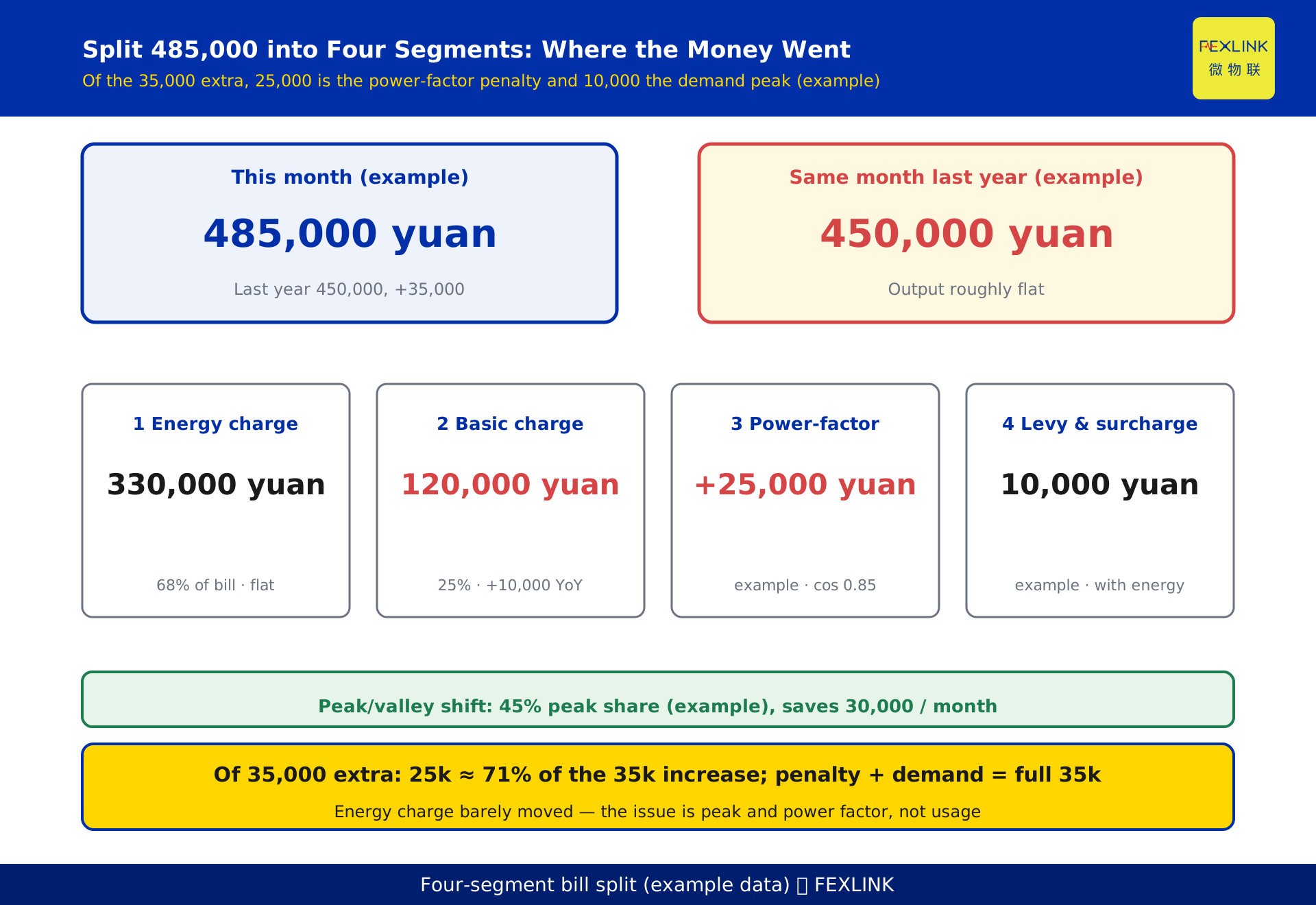
A plant's last-month bill was 485,000 yuan; a year earlier it was 450,000 yuan. Production was essentially flat, yet it spent 35,000 yuan more. Splitting the 485,000 into four segments:
- Energy charge: 330,000 yuan, 68% of the bill, unchanged from last year.
- Basic charge: 120,000 yuan, 25%, up 10,000 yuan from last year.
- Power-factor adjustment: +25,000 yuan (surcharge); last year it was exactly at threshold, 0.
- Levy & surcharge: 10,000 yuan, unchanged from last year (government funds and surcharges levied with the energy tariff; no change here).
- Peak/valley spread: current peak-hour share is about 45%; shifting to valley hours could save an estimated 30,000 yuan per month (opportunity item, not in the current bill). The four items sum to exactly 485,000 yuan.
Of the 35,000 yuan extra, 25,000 is the power-factor penalty and 10,000 is the basic charge pushed up by the demand peak — these two make up the full 35,000-yuan increase; the penalty alone is about 71% (25,000÷35,000) of the increase. The energy charge barely moved. The problem is not "using more"; it is "peak power and power factor."
3. Locating the demand peak from the records
When the basic charge rises, do not blame the equipment yet — look at the meter's demand curve. (How demand is defined is covered head-on in KD-0468; this article only teaches you to reverse-locate that peak from a bill anomaly.)
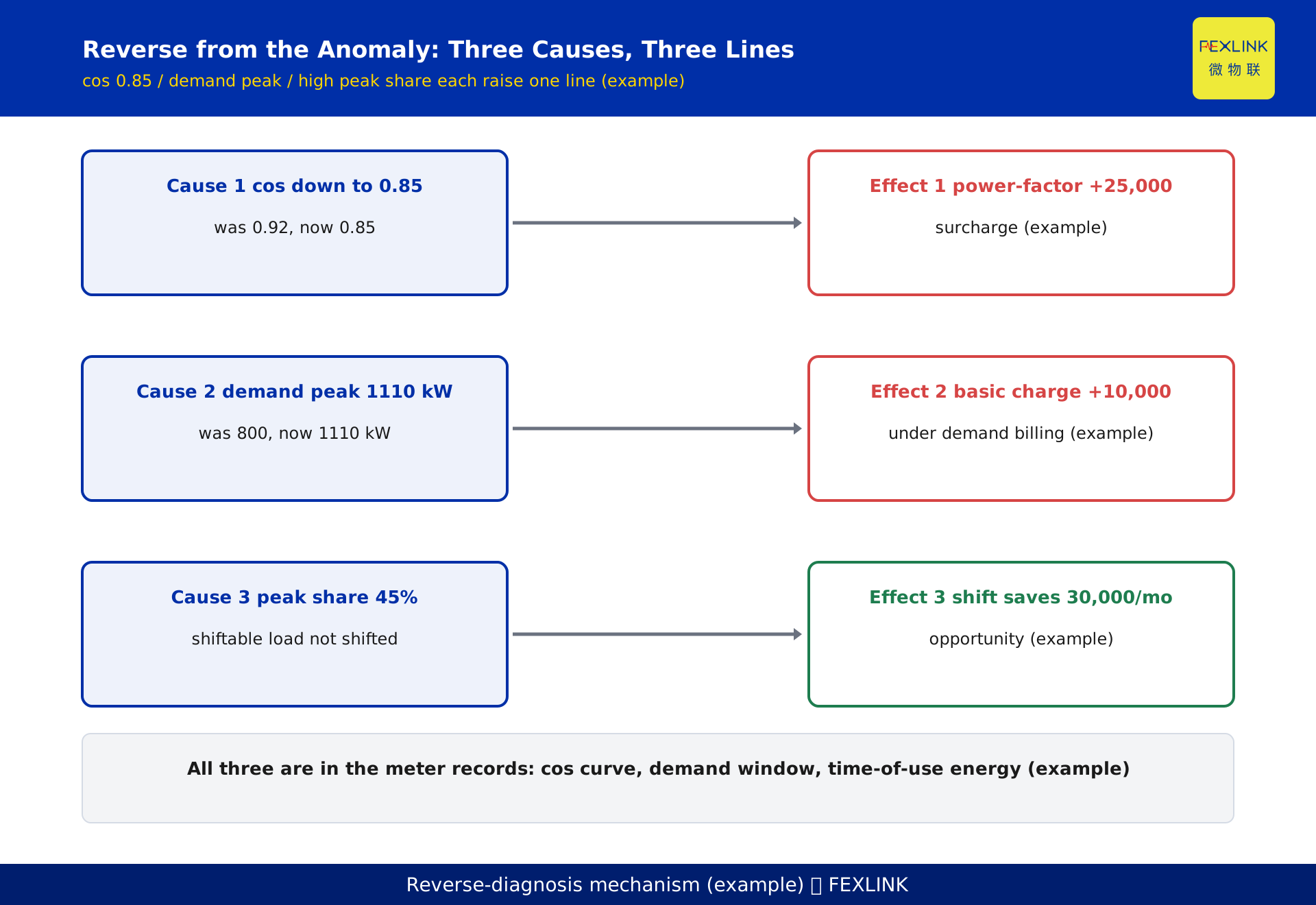
Demand is the largest 15-minute average power within the billing period. On a typical two-part tariff the basic charge is billed monthly, but if you are on demand billing, one or two spike windows decide the entire month's basic charge. In this example demand rose from 800 kW to 1110 kW; at the illustrative rate of 32 CNY/kW·month that is about 10,000 yuan extra per month (9,920 yuan) — the main reason the basic charge rose 10,000 yuan year on year.
How to locate it: pull the meter's demand curve (one point every 15 minutes) and find where the monthly maximum occurs — which day, which hour. If the spike clusters around a particular machine start-up or a production line switching on together, you have a concrete handle to flatten it. The ESA all-element smart meter records the demand curve per circuit, so you can export that spike directly at month-end instead of inferring it from the main meter.
4. Power factor below threshold: which loads are dragging it down
The power-factor surcharge roots in cos φ dropping. Here cos φ fell from 0.92 to 0.85, which directly triggered the 25,000 yuan surcharge.
Common loads that pull power factor down fall into a few classes. First, rectifier-type equipment — variable-frequency drives, rectifier power supplies, switch-mode power supplies — draw non-sinusoidal current from the grid and carry large reactive power. Second, intermittent or impact loads such as welding machines, electric-arc furnaces, and medium-frequency furnaces. Third, large quantities of fluorescent lamps or LED drivers without local compensation also drag it down. A plant that adds VFDs but skips reactive compensation typically sees cos φ drop first and get penalized after.
To tell whether a load is the culprit, read the cos φ record from the meter or monitor by time segment. If the worst drop coincides with a certain type of equipment running, the corrective direction is clear. The ESE power-quality monitor logs cos φ and harmonics over time, so in the monthly review you can state exactly which device pulled the power factor down.
5. How much headroom is left in peak/valley shifting
The fourth segment, the peak/valley spread, is not a penalty but an opportunity. In this example the peak share is 45%. Assuming a peak tariff of 1.20 CNY/kWh and a valley tariff of 0.38 CNY/kWh (both constructed examples, subject to the local tariff document), moving part of the shiftable load to valley hours could save about 30,000 yuan per month.
Shifting is not stopping production; it is rescheduling deferrable processes — non-continuous compressed air, pre-cooling for refrigeration, charging, water treatment — into valley hours. The size of the opportunity is read from the time-of-use energy mix: the higher the peak share and the more shiftable load you have, the larger the space. This step is computable from the ESA time-of-use energy records without a complex system.
6. The four-segment reverse-diagnosis method
String the above into a reusable reverse-diagnosis routine, run it every month:
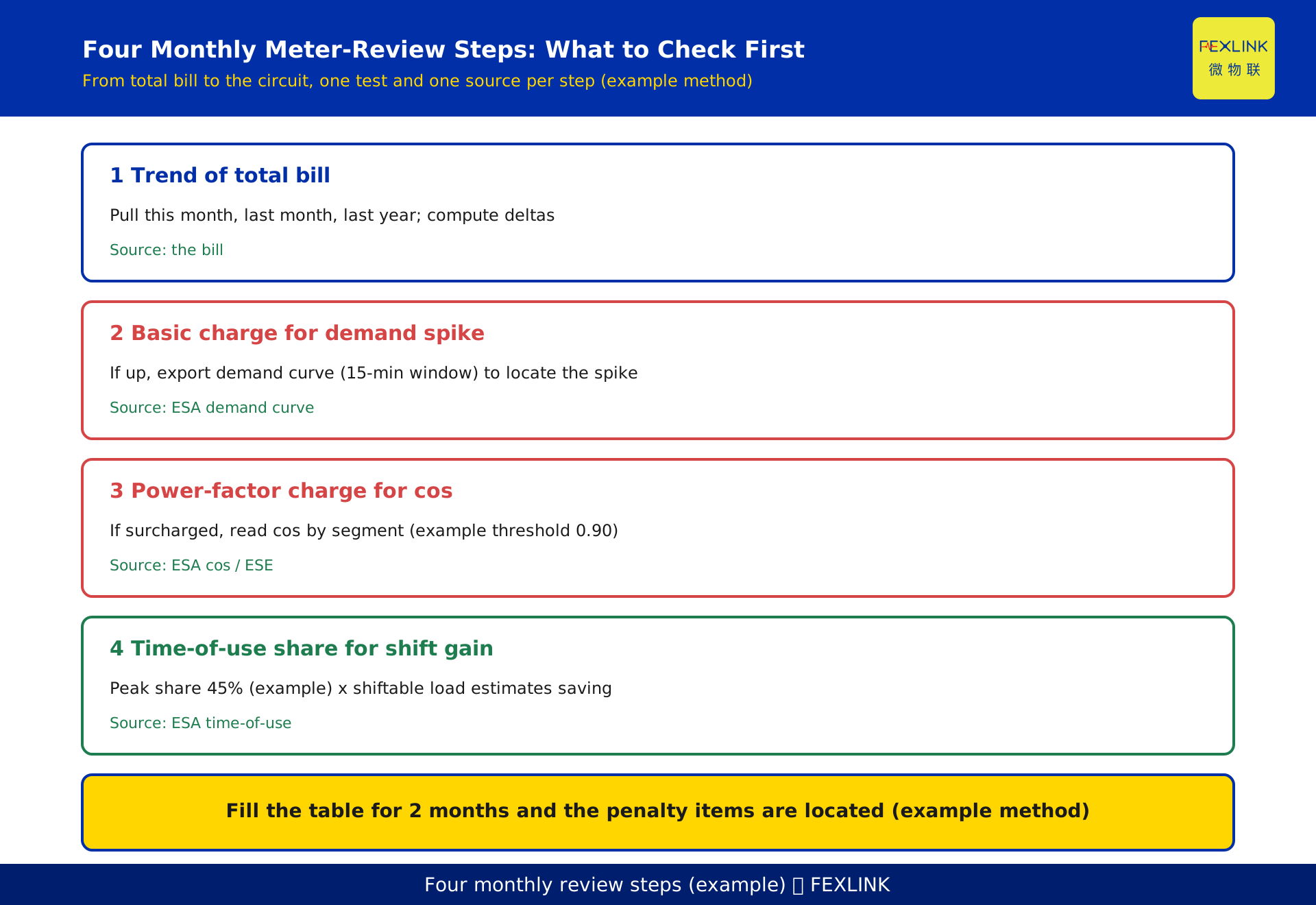
Step 1, pull the total. Take this month's bill alongside last year's same month and last month; compute the period-over-period and year-over-year deltas. Step 2, split the four segments. Fill in energy charge, basic charge, power-factor adjustment, and peak/valley spread; see which segment the delta landed in. Step 3, reverse the basic charge. If it rose, export the demand curve and find the spike (the 15-minute window maximum), locating it to a device or time slot. Step 4, reverse the power-factor charge. If there is a surcharge, read the cos φ record and find the lowest segment by time, mapping it to a specific load. Step 5, size the shift opportunity. Read the time-of-use energy share and estimate the shiftable load's savings. Step 6, write the conclusion. State clearly "the extra money = which segment + which device + how much," then track it next month.
Run it for two months and the penalty items are essentially all located.
7. Building the monthly bill-review table
For the method to stick, you need one fixed table, filled and compared every month. Suggested columns:
- Month, total bill, period delta, year delta.
- Energy charge (kWh, amount, peak/flat/valley share).
- Basic charge (billing basis, maximum demand in kW, amount).
- Power-factor adjustment (monthly average cos φ, compliant or not, surcharge/credit amount).
- Shift savings (shiftable load, estimated saving).
- This month's conclusion and next month's action.
Data sources: the total and segments come from the bill; maximum demand, cos φ, and time-of-use energy come from the ESA all-element smart meter's exported records; harmonic and power-quality detail comes from the ESE power-quality monitor. The same table every month, filled for 2 months in a row, already shows the trend.
8. How the products fit: the roles of ESA and ESE
This diagnostic is data-driven, and the data comes from metering at the edge.
The ESA all-element smart meter (full name: ESA all-element smart meter, capable of per-circuit voltage, current, power, demand, and time-of-use energy acquisition) archives the demand curve and cos φ records month by month; it is the data base for steps three, four, and five. Whether the basic-charge spike and the power-factor surcharge can be located depends on whether this meter records, and how finely.
The ESE power-quality monitor (full name: ESE power-quality monitor, focused on harmonics, voltage fluctuation, and power-factor measurement) clarifies which device pulled cos φ down and which circuit the harmonics came from; it is the fine-grained probe for power-factor diagnosis.
Together with the digital electrical intelligent supervision system, they connect the chain "bill anomaly → demand/power factor → specific circuit," turning the review from flipping paper bills into reading curves.
9. Frequently asked questions (FAQ)
Q: If the bill went up, does that mean we used more electricity?
Not necessarily. In this example production did not grow and the energy charge was flat; the extra 35,000 yuan was entirely in the basic charge and the power-factor charge. Judge by the four-segment split, not the grand total.
Q: How is the power-factor charge calculated — could the utility have made a mistake?
The power-factor adjustment is assessed on power factor: credit when compliant, surcharge when not; the mechanism is public. What you should do is verify whether your own cos φ record truly fails, not doubt the formula. The exact credit/penalty ratios follow the local current document; this article lists no numbers.
Q: Is power factor 0.90 a hard standard?
0.90 is a common assessment value for many large industrial customers, but local and sector rules differ and it floats with capacity class. The governing value is the assessment standard published by the local utility; this article uses 0.90 only as an illustrative threshold.
Q: Is a main meter enough to run this diagnosis?
No. Both the basic-charge spike and the power-factor diagnosis need circuit-level data: the demand curve must locate the device, and cos φ must be read by time segment. At minimum, fit the main energy circuits with meters that record demand and cos φ.
Q: Can two months show a result?
Yes. The diagnosis itself is "finding the problem" and needs no retrofit. Month one builds the table, splits the four segments, and locates the penalty items; month two validates the trend and lists actions. What pays off first is "seeing the bill clearly," not "saving instantly."
Scope and limitations
- The four-segment reverse-diagnosis method applies to large industrial and general commercial customers on a two-part tariff; single-part tariff customers may skip the basic-charge and demand portions.
- The example figures in this article (total bill 485,000 yuan, demand 800→1110 kW, cos φ 0.92→0.85, power-factor surcharge 25,000 yuan, etc.) are constructed solely to illustrate the method and represent no real customer or project; actual values must come from the on-site bill and meter records.
- The power-factor assessment standard (e.g., 0.90) follows the local utility's current document. This article cites no standard clauses and gives no specific credit/penalty ratio for the power-factor adjustment; all such ratios are per the local document.
- The peak tariff of 1.20 CNY/kWh and valley tariff of 0.38 CNY/kWh are constructed illustrative prices, used only to show the order of magnitude of shift savings; actual prices follow the local tariff document.
- The illustrative demand rate of 32 CNY/kW·month and capacity rate of 23 CNY/kVA·month are constructed examples representing no real regional price; the billing basis and rates follow the local document.
- The specific models and parameters of the ESA all-element smart meter and the ESE power-quality monitor follow the latest selection manual and product knowledge base; this article is not a selection or procurement recommendation.
Frequently Asked Questions
Your Bill Keeps Growing for No Reason
When production is flat but the bill keeps climbing, the extra money is almost always in two places: the demand-related portion of the demand charge