 FEXLINK Research Institute
Direct Answer
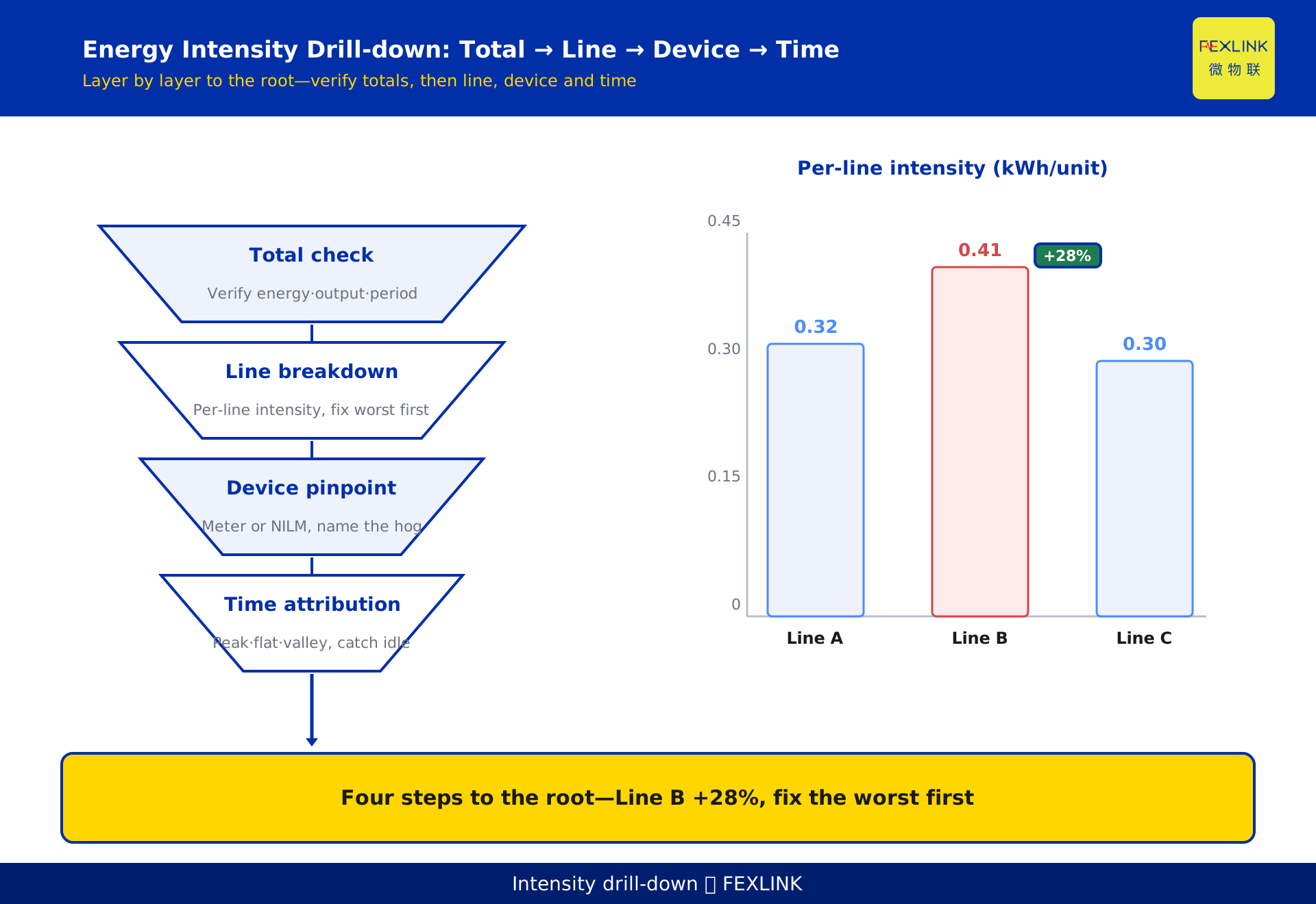
Why is your unit consumption higher than your peers on the same production line? Dig down through the data: High unit consumption is not "one cause" but a chain of causes—dig down: check the total, look at the structure, then locate the equipment and the time period. Unit consumption = total energy ÷ output. Dig in four steps: total verification, line breakdown, equipment location, and time attribution. Dig to the bottom and the root cause shows itself.
A scenario: A plant's unit consumption was 12% higher than peers—they dug into the data: the total was not high—one line had unbalanced shifts—the night shift idled too much. The logic is that high unit consumption requires digging down—from the total to the structure, the root cause is in the details.
An analogy — High unit consumption is like a fever: fever medicine treats the symptom—you need to find the lesion. Data drilling is like a medical check: examine layer by layer until you find the inflammation.
1. The First Question: Is the Total Correct?
Check the total first — is the total energy data accurate: is metering complete? Is the output figure correct: piece-count or time-based? Do they match: is the statistical period consistent? The cost of a wrong total — wrong data leads to wrong benchmarking; wrong calibration makes comparison meaningless; a wrong period turns fluctuation into a problem; How to verify — compare with the electricity bill; check the output ledger against the MES; check the statistical period for a consistent monthly basis; Then what — if the total is right, move to structural analysis; if it is wrong, fix the data before benchmarking.
In one sentence: the first step of drilling is to verify the total—energy, output, and calibration must align—if the data is wrong, all analysis is useless.
Total verification table:
| Check | Method | Standard |
|---|---|---|
| Energy | Compare bill | Consistent |
| Output | Compare MES | Consistent |
| Calibration | Check period | Aligned |
An example — A plant had abnormally high unit consumption—first they verified the total: energy matched the bill and output matched the MES—the data was right, so they moved on. The logic is that the total is the "foundation"—confirm the data first, then dig—if the data is wrong, fix it first.
Common pitfalls of total verification — checking only one table: energy right, output missed; misreading meters: the data looks right but is wrong; verify both data sets when checking the total.
2. The Second Step: Line Breakdown
What line breakdown means — split the total unit consumption into each line: per-line unit consumption—find the difference: which line pulls up the whole; How to break down — per-line metering: each line has its own meter; per-line output: each line has its own statistics; calculate per-line unit consumption and compare to find the gap; Sources of difference — equipment age: different efficiency; load rate: high load means lower unit consumption; idling: low load means high unit consumption; What you see after the breakdown — the distribution of unit consumption: high and low; the ranking of differences: dig into the worst first; The precondition — per-line metering in place: independent meters; per-line output clear: independent statistics—only then is the breakdown accurate.
In one sentence: line breakdown finds the "lagging" line—measure per line, calculate per line—rank the differences and dig into the worst first.
Line difference table:
| Line | Unit consumption | Difference |
|---|---|---|
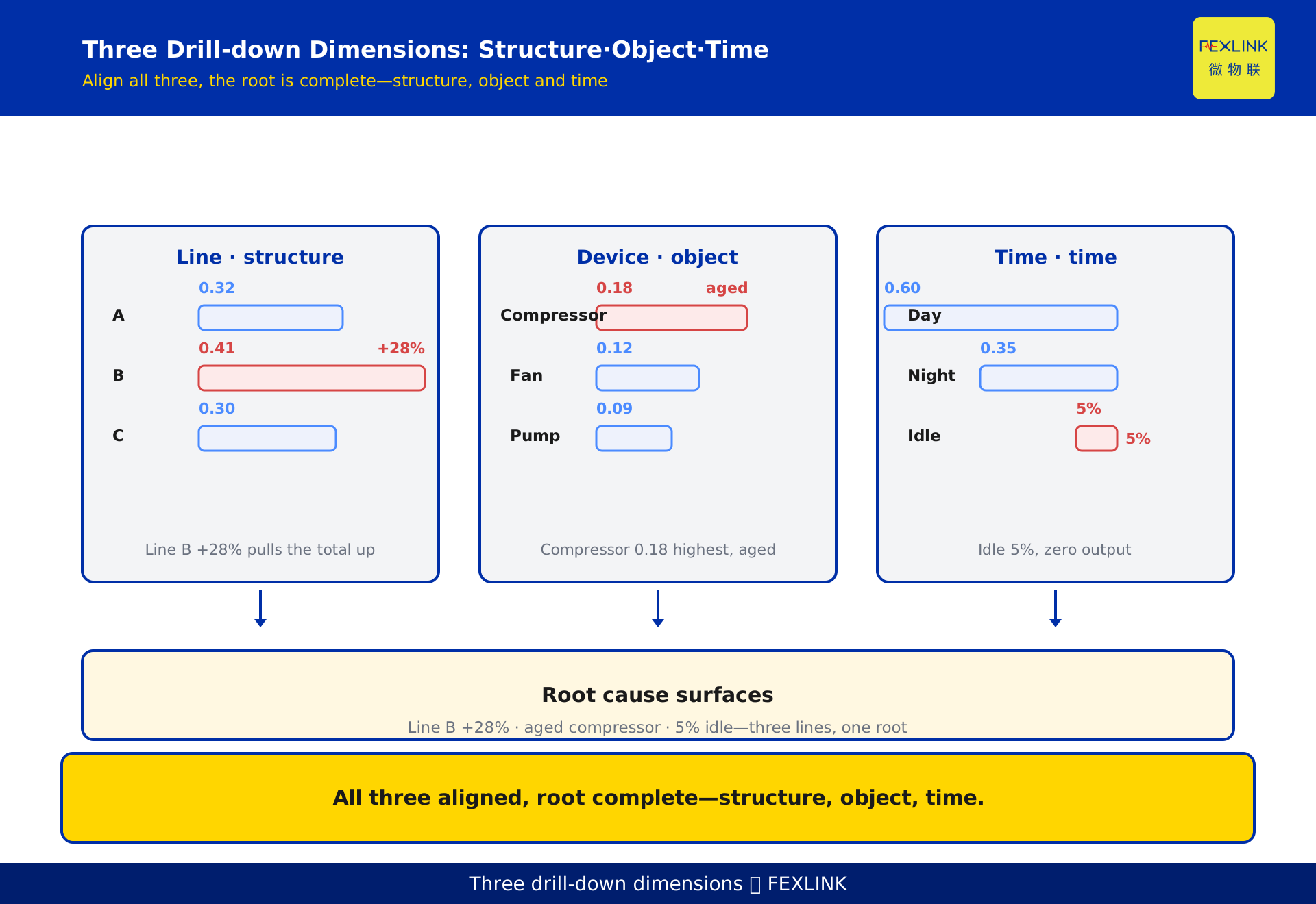
| Line A | 0.32 | Baseline |
| Line B | 0.41 | +28% |
| Line C | 0.30 | -6% |
An example — A plant broke down the lines: Line A was 0.32, Line B was 0.41—Line B pulled up the whole—they focused on Line B for drilling. The logic is that breakdown is "location"—compare line by line, the lagging line appears—dig into the worst first for the best return.
3. The Third Step: Equipment Location
What equipment location means — split the line unit consumption into equipment: which machines consume the most—find the high-consumption equipment: those with low efficiency; How to see equipment — per-equipment metering: install meters on large machines; NILM load disaggregation: split without meters; equipment unit consumption: output vs. power; Causes of high consumption — aging: efficiency drops; improper loading: a big machine doing a small job; faults: hidden losses; The output of location — an equipment list ranked by unit consumption; the priority targets: the worst equipment; Getting equipment data — large equipment metered directly: most accurate; small equipment via load disaggregation: lower cost—combine both for full coverage.
In one sentence: equipment location finds the "power guzzlers"—meter per equipment or use load disaggregation—rank by unit consumption and handle the worst first.
Equipment location table:
| Equipment | Unit consumption | Status |
|---|---|---|
| Compressor | 0.18 | Aging |
| Fan | 0.12 | Normal |
| Pump | 0.09 | Low load |
An example — A plant drilled into Line B equipment: the compressor had the highest unit consumption—the check showed aging and lower efficiency—it was listed for retrofit. The logic is that location "names" the target—rank equipment unit consumption and name the high consumers—retrofit has an object and investment has a return.
4. The Fourth Step: Time Attribution
What time attribution means — split equipment consumption into time periods: when is consumption high—find idling: equipment still running during low-output periods; How to see time periods — per-period metering: peak, flat, and valley; equipment start-stop compared with the production rhythm; idling identification: low output but continuous consumption; Sources of idling — shift handover: equipment not shut down; standby not off: waiting for materials or orders; unscheduled running: running without orders; The output of attribution — an idling period list: from when to when; the idling loss: how much electricity bill was wasted; The source of time data — time-of-use meters: automatic peak/flat/valley split; platform minute-level data: period aggregation—clear sources make attribution credible.
In one sentence: time attribution catches "idling"—look at consumption by period and compare with the production rhythm—name the idling periods and calculate the loss.
Period distribution table:
| Period | Consumption | Output |
|---|---|---|
| Day | 60% | High |
| Night | 35% | Medium |
| Idling | 5% | Zero |
An example — A plant did time attribution: equipment consumed 5% during standby with zero output—machines were not shut down at shift change—rules plus automatic shutdown solved it. The logic is that attribution "catches it in the act"—compare periods, idling appears—calculate the loss precisely, and measures become targeted.
The Combination: Root Cause Appears
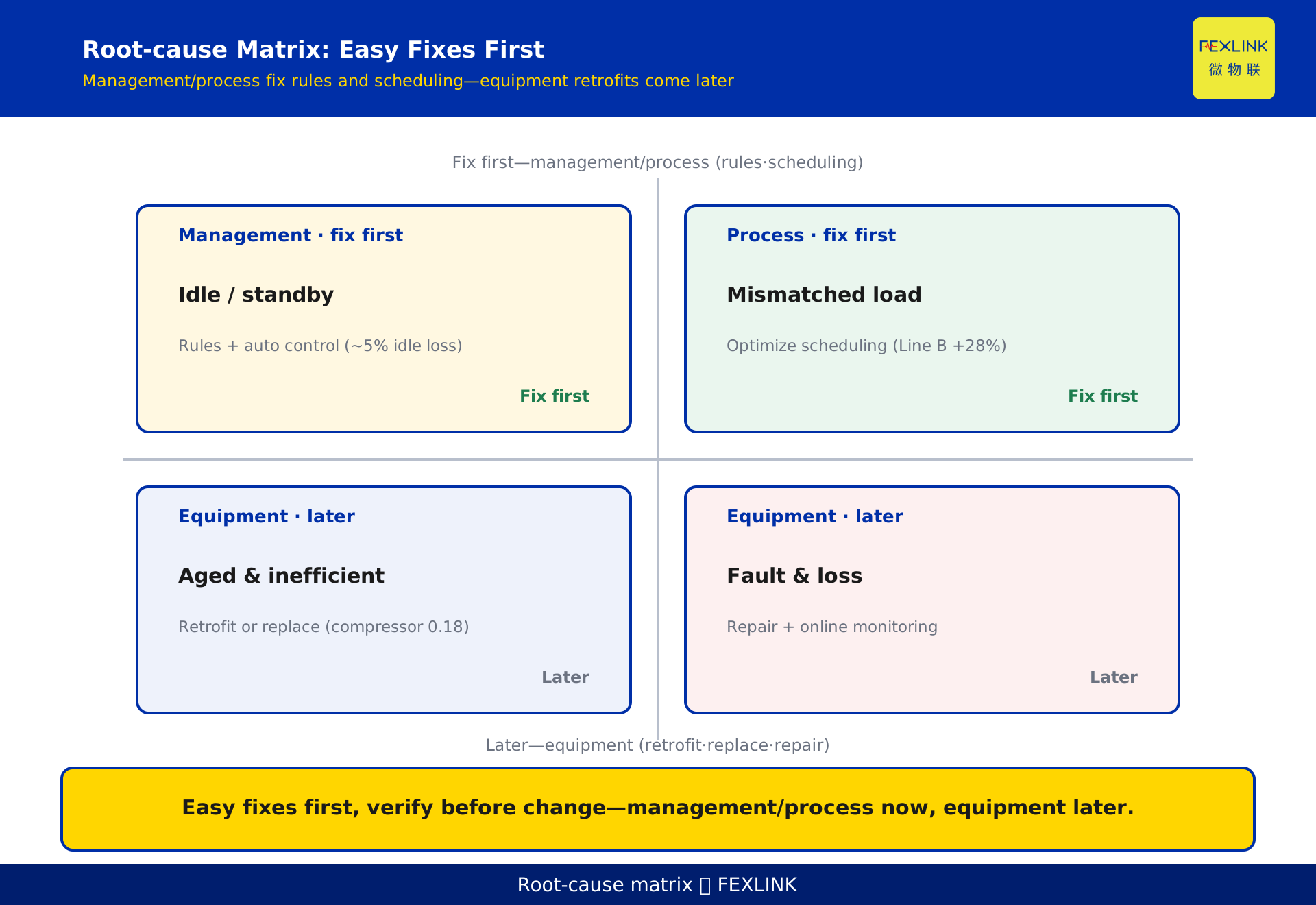
The four steps in series — verify the total, break down the lines, locate the equipment, attribute the time—dig layer by layer until the root cause appears; The types of root causes — management: idling and standby not off; equipment: aging and low efficiency; process: improper loading and unreasonable rhythm; How to verify a root cause — check against data: the cause explains the difference; small-scale verification: change one thing and see the effect; data confirmation: did unit consumption drop; The priority of root causes — easy first: management issues first; return on investment: high-return actions first; risk ranking: safety-related items first; The rhythm — fast first, detailed later: the total verifies fast, equipment location is detailed—keep the four steps connected without stopping—record each step for traceability.
In one sentence: the four steps in series dig to the bottom—management, equipment, and process root causes—verify before changing, easy first.
Root cause classification table:
| Type | Symptom | Action |
|---|---|---|
| Management | Idling/standby | Rules+automation |
| Equipment | Aging/inefficient | Retrofit |
| Process | Improper load | Optimize rhythm |
An example — A group did the four-step drill: total verified, Line B identified, compressor located, idling caught—the root causes were aging plus standby—retrofit and rules together. The logic is that the combination is "systematic digging"—four steps in series, the root cause is complete—handle by type, and investment becomes precise.
6. How Data Supports the Drill
Where the data comes from — per-line and per-equipment metering: meters in place; load disaggregation: NILM splits without meters; platform aggregation: unified calibration; The granularity of drilling — line level: per-line unit consumption; equipment level: per-machine consumption; time level: peak/flat/valley distribution; The support tools — the energy-efficiency benchmarking system: baseline and difference; the energy diagnosis solution: drilling path and methods; the platform dashboard: one screen to the bottom; The drilling cycle — monthly routine: track unit consumption fluctuation; quarterly depth: equipment-level diagnosis; annual review: root cause handling status.
In one sentence: drilling depends on data—metering in place, disaggregation as backup, platform aggregation—fine granularity makes root causes findable.
Support tools table:
| Step | Tool | Role |
|---|---|---|
| Metering | ESA meter | Per line/equipment |
| Disaggregation | Tianyan E-01 | NILM splitting |
| Analysis | Benchmarking | Baseline/difference |
An example — A park built a drilling system: ESA meters measured per line and per equipment, Tianyan E-01 load disaggregation covered the rest, and the benchmarking system provided the baseline—drilling in one step. The logic is that support is a "tool chain"—metering, disaggregation, and analysis link together—with the chain complete, root causes can be dug out.
Back to the ESA family — this is how the solution lands: the ESA full-element smart meter provides per-line and per-equipment metering, Tianyan E-01 (NILM load disaggregation) splits equipment-level data without extra meters, the energy-efficiency benchmarking system provides the baseline and differences, and the energy diagnosis solution provides the drilling path—from the total to the root cause, one chain.
Scope and Limitations
- The conclusions in this article are intended for LV distribution and electrical-safety sites. Standard numbers (GB/T 2589) refer to their currently effective editions, and product parameters follow the latest FEXLINK selection handbook and product knowledge base.
- Quantitative criteria (protection zone, discharge and residual voltage, earth resistance, thresholds and grading) hold under the preconditions stated in this article. Where the site voltage level, earthing arrangement, environmental category or load profile differs, the figures must be recalculated. Specific configurations involving Tianyan E-01 (NILM load disaggregation), ESA all-element smart meter should be verified against actual circuit parameters.
- Specific product models and parameters are subject to the latest selection handbook and product knowledge base; this article does not constitute selection or procurement advice.
- Standard numbers cited here refer to the currently effective editions; when a standard is revised, the related quantitative conclusions must be re-checked.
- Deployment and implementation for specific projects must be carried out by qualified engineers based on site survey and design drawings.
Frequently Asked Questions
Why Is Your Line's Specific Energy Consumption Higher
Dig down through the data: High unit consumption is not "one cause" but a chain of causes—dig down: check the total, look at the structure