 FEXLINK Research Institute
Direct Answer
How to design a plan that cuts both the demand charge and the TOU bill? The joint optimization takes the "demand curve + TOU tariff" as the input and schedules on the time dimension — the shiftable load is arranged into the valley and an automatic demand ceiling is preset before the sharp peak to shed load — satisfying the double goal of "the peak stays under the demand threshold and the energy falls into the valley as much as possible" — the landing relies on three layers: the TIANYAN E-06 predicts the load curve, the energy supervision center dispatches the schedule and the FECB2SP/SLP smart breakers execute the shedding.
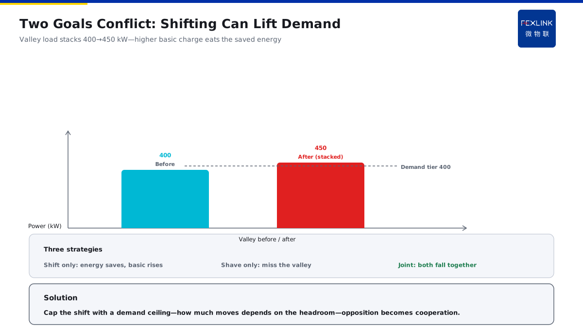
A scenario: A company only cares about moving the peak — it schedules all the large devices into the valley — but the valley power stacks up and the demand soars — the extra basic charge is larger than the money saved in the valley — the two goals fight each other. The logic is that the demand goal and the TOU goal conflict by nature — moving the peak squeezes the load into the valley and the valley power stack raises the demand — shedding the demand misses the cheap valley — to cut both, the schedule must be joint — see the conflict first, then the plan.
1. Why the Demand and TOU Goals Conflict
The demand goal — the peak stays under the demand threshold: crossing the threshold raises the whole-month basic charge to a higher band; The TOU goal — the energy falls into the valley as much as possible: moving the energy from the peak to the valley cuts the energy bill; The source of the conflict — moving the peak squeezes the load into the valley: the valley power stacks and the demand peak may be pushed up; The consequence of the conflict — caring about one side only: moving the peak saves the energy bill but raises the basic charge; shedding the demand saves the basic charge but misses the cheap valley.
In one sentence: the demand manages the "peak height" and the TOU manages the "energy position" — moving the peak changes the position and may raise the peak — the two goals must be optimized together, not each on its own.
The comparison table of the conflicting strategies:
| Strategy | Energy bill (TOU) | Basic charge (demand) | Net effect |
|---|---|---|---|
| Move the peak only | Save | May pay more | Offset each other |
| Shed the demand only | No saving | Save | Miss the valley |
| Joint schedule | Save | Save | Both down |
An example: A company compares two schemes — scheme A only moves the peak, the valley power stacks and the demand hits 450 kW with more basic charge; scheme B schedules jointly, the moved energy is limited by the demand headroom and the demand stays at 400 kW with both bills falling — scheme B saves 3,000 yuan more per month. The logic is that the joint schedule earns the "no band-jump" money that the single-goal strategy loses — the demand headroom limits the moved total and both goals are met — the comparison shows the advantage of the joint plan.
2. The Inputs of the Joint Optimization: Load Curve + Tariff + Demand Ceiling
The load curve — the 24-hour load curve: the full picture of the power in each period; The TOU tariff — the prices of the sharp/peak/flat/valley periods: how cheap the valley is and how expensive the peak is; The demand ceiling — the band threshold of the basic charge: crossing which line makes the basic charge jump a band; The constraints — the process constraints, shiftable durations and interruption boundaries: the hard limits the schedule cannot violate.
In one sentence: the load curve knows "where the electricity is", the tariff knows "where it is cheap" and the demand ceiling knows "where it cannot exceed" — the three inputs give the schedule its basis.
A company receives the three inputs — the load curve shows the 9-11 peak, the tariff shows 0.35 yuan valley and 1.15 yuan peak and the ceiling is 400 kW — the platform schedules by first satisfying the demand ceiling and then chasing the valley energy — the order cannot be reversed.**
3. The Scheduling Logic of the Valley Production and the Sharp-Peak Demand Shedding
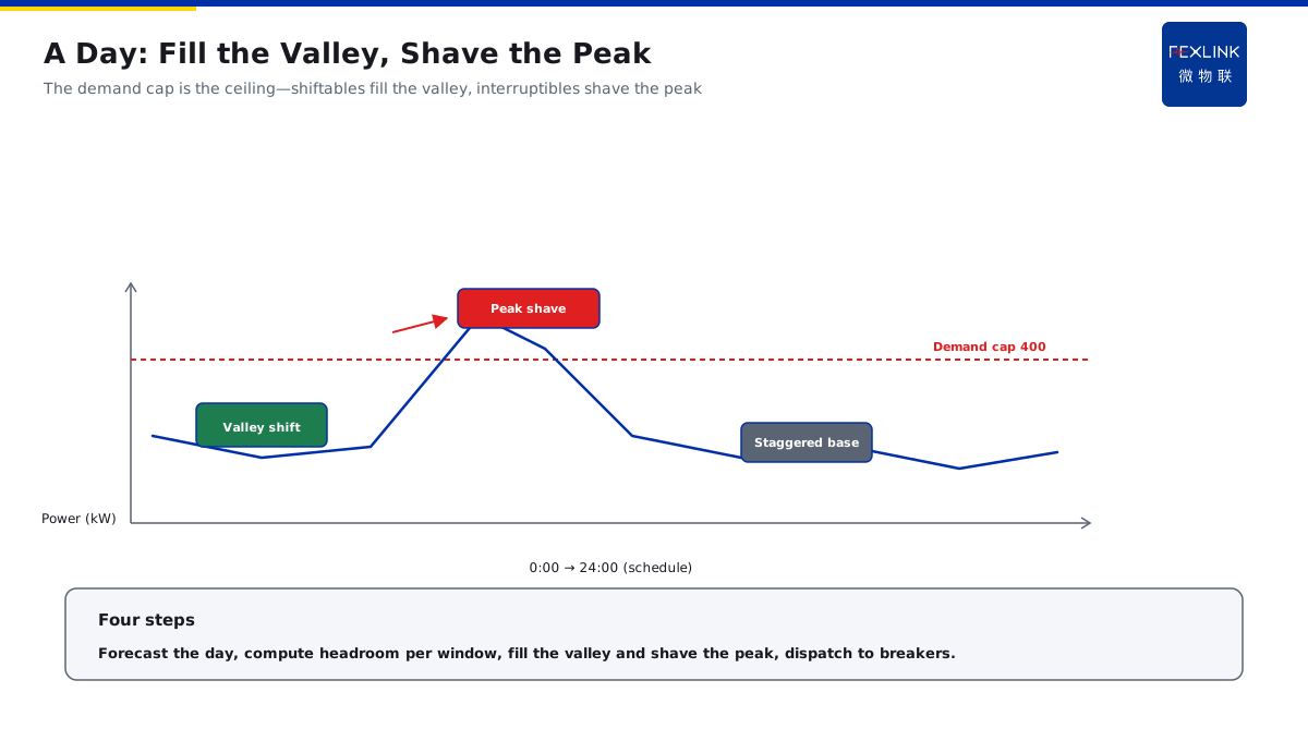
The valley production — the shiftable load is scheduled into the valley: charging and storable steps run in the cheap period; The sharp-peak shedding — the power is limited in the sharp-peak period: the ceiling is preset and the load is shed automatically when exceeding; The scheduling principle — move the shiftable first, limit the interruptible next and stagger the non-shiftable last: scheduled by the flexibility priority; The scheduling constraint — the valley power cannot break the demand ceiling: the moved total is limited by the demand space.
In one sentence: the valley "fills" the energy and the sharp peak "sheds" the power — filling cannot break the ceiling and shedding prioritizes the interruptible — the schedule is a fill-and-shed on the time axis.
The four-step scheduling process — step one: predict the 24-hour load curve and mark the sharp-peak windows; step two: with the demand ceiling as the cap, calculate the demand headroom of each period; step three: fill the shiftable load into the valley headroom and place the interruptible load at the sharp-peak shed positions; step four: dispatch the schedule to the smart breakers for automatic execution — four steps, the schedule is closed.
An example: A day schedule of a company — the valley 0-6 arranges the charging piles and ice makers (shiftable) — the sharp peak 9-11 sets the 400 kW ceiling and automatically sheds the air-conditioning (interruptible) — the reactors (non-shiftable) run continuously and only stagger at the start. The logic is the fill-and-shed time schedule — the valley fills the shiftable, the sharp peak sheds the interruptible and the non-shiftable staggers as the base — the three classes each in their place and the double goal is met at the same time.
4. How the Automatic Demand Control Is Embedded
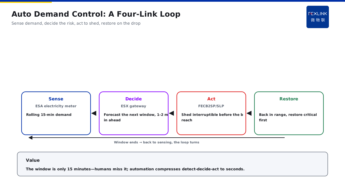
The sensing layer — the ESA meter collects the demand in real time: the current demand is calculated by the rolling 15-minute window; The decision layer — the ESX edge gateway judges the overshoot risk: predicting whether the next window will cross the demand ceiling; The execution layer — the FECB2SP/SLP smart breakers shed the load automatically: cutting the interruptible load before the overshoot; The loop — sense-decide-execute-recover: the load recovers after the demand falls, forming an automatic loop.
In one sentence: sense the real-time demand, decide the overshoot risk, execute the automatic shedding and recover automatically — the automatic demand control is a four-link loop.
The timing details of the automatic control — the sensing cycle: the demand window rolls every 15 minutes and the sensing never stops; the decision lead: the gateway predicts the next-window demand and judges the overshoot 1-2 minutes ahead; the execution order: cut the interruptible first, limit the shiftable next and never touch the non-shiftable; the recovery strategy: after the window demand falls, recover in the "critical-load-first" order — the timing details decide the success of the control.
The value of the automatic control — the demand window is only 15 minutes — with manual finding, notification and execution, the window is long gone — the automatic control compresses "find-decide-execute" to the second level — only then the shedding catches up with the window.
An example: A company sets the 400 kW ceiling — the window at 9:10 hits 395 kW — the ESX gateway predicts the next window will cross — the FECB2SP breaker automatically sheds the air-conditioning compressor — the demand falls to 360 kW — the window ends and the load recovers automatically. The logic is the timeliness of the automatic control — by the time a human finds the overshoot and cuts, the window has passed — the gateway predicts and the breaker executes, cutting within the window — the sense-decide-execute loop makes the demand shedding in time.
5. The Effect Measurement and the Payback Period of the Plan
The measurement inputs — the moved energy, the valley spread and the demand band difference: the three variables decide the benefit; The measurement formulas — the energy-bill saving = the moved energy × the spread; the basic-charge saving = the demand band-down × the band difference; The measurement period — the payback period = the retrofit investment ÷ the monthly saving: the payback is counted by the monthly benefit; The measurement verification — a one-month trial run: compare the bills before and after the optimization to verify the measurement.
In one sentence: the energy bill saves on "the spread × the energy" and the basic charge saves on "the band-down × the band difference" — the payback period = the investment ÷ the monthly saving — the trial run verifies the measurement.
The measurement steps — step one: calculate the energy-bill saving, the moved energy × the weighted spread of each period; step two: calculate the basic-charge saving, the demand band-down × the band difference; step three: add up the monthly saving, the energy bill + the basic charge; step four: calculate the payback period, the investment ÷ the monthly saving — four steps, the measurement is complete.
An example: A company measures — moving 200 kWh per day with an 0.8 yuan spread — the energy bill saves 160 yuan per day; the demand falls from 450 kW to below 400 kW with a 20 yuan/kW band difference — the basic charge saves 1,000 yuan per month — about 5,800 yuan saved per month in total — the retrofit investment is 150,000 yuan — the payback period is about 26 months.**
Back to the overall architecture of the energy supervision center plan — the sensing layer: the ESA meter collects the load and demand curve; the prediction layer: the TIANYAN E-06 predicts the 24-hour load and the peak windows; the scheduling layer: the energy supervision center generates the schedule with the demand ceiling as the hard constraint and the valley energy as the soft goal; the execution layer: the FECB2SP/SLP smart breakers shed the load automatically by the schedule — the four layers of sense-predict-schedule-execute close the joint optimization. The phased landing path — phase one: build the load ledger and the demand curve to know the shiftable and interruptible load; phase two: go live with the TIANYAN E-06 load prediction and mark the sharp-peak windows; phase three: deploy the ESX gateway and the FECB2SP/SLP breakers to close the automatic shedding loop; phase four: run the valley production on trial and fully commission the joint optimization — the four phases advance gradually, the investment is phased and the benefit comes early.**
Scope and Limitations
- The conclusions in this article are intended for LV distribution and electrical-safety sites. Criteria are compiled from public codes and FEXLINK product documentation, and product parameters follow the latest selection handbook and product knowledge base.
- Quantitative criteria (protection zone, discharge and residual voltage, earth resistance, thresholds and grading) hold under the preconditions stated in this article. Where the site voltage level, earthing arrangement, environmental category or load profile differs, the figures must be recalculated. Specific configurations involving FECB2SP/SLP smart breaker, ESX edge gateway, Tianyan engine E-06 should be verified against actual circuit parameters.
- Specific product models and parameters are subject to the latest selection handbook and product knowledge base; this article does not constitute selection or procurement advice.
- Standard numbers cited here refer to the currently effective editions; when a standard is revised, the related quantitative conclusions must be re-checked.
- Deployment and implementation for specific projects must be carried out by qualified engineers based on site survey and design drawings.
Frequently Asked Questions
Cutting Both the Demand Charge and the TOU Bill
The joint optimization takes the "demand curve + TOU tariff" as the input and schedules on the time dimension — the shiftable load is arranged into the