 FEXLINK Research Institute
Direct Answer
How to build the energy-saving diagnosis for the small and medium factory? By the "key-circuit sub-metering + NILM load disaggregation + SEC benchmarking" light scheme — the reactive and the idle waste first, then the rolling expansion — the limited budget still lands and saves — the consultant audit expensive and once a year, a continuous online tool better — 2 weeks the survey, 3 months the verification, the savings quantified and the list executable.
A scenario: The factory owner wants to save — the consultant audit hundreds of thousands, once a year — no tool by himself — the end, nothing. The logic is that the diagnosis needs "the light and sustainable" — the sub-metering base, the disaggregation finds, the benchmarking sees — the high-certainty first, the savings out.
An analogy — The diagnosis like the physical: the blood pressure first (the data), the index over the standard (the analysis), the prescription last (the list) — the cheap and the continuous, the disease prevented.
1. The Three Layers (Collection/Analysis/List)
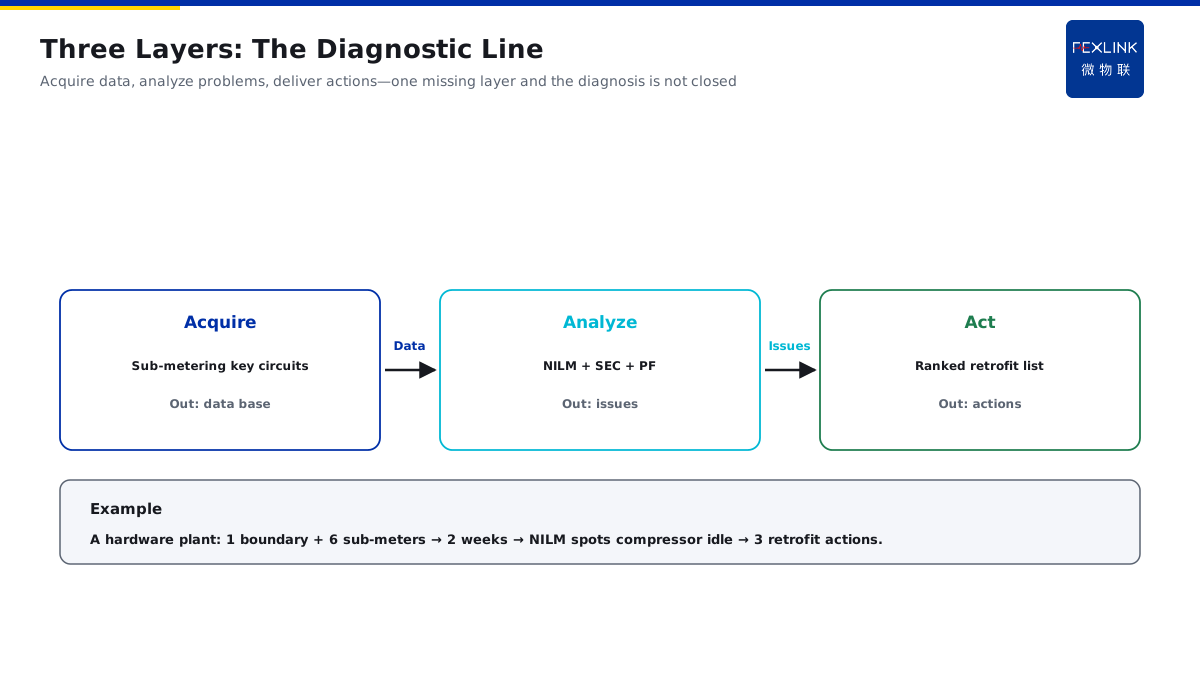
The three layers — the collection (the meters) + the analysis (the disaggregation and the benchmarking) + the list (the renovation) — each its duty; The collection — the key circuits: the total + the AC/power/lighting — the base; The analysis — the NILM + the SEC benchmarking + the power factor — the problems; The list — by the certainty, each with the savings and the payback.
In one sentence: the three layers = the collection-analysis-list — the data in, the problems out and the list ordered — the closed, the diagnosis lands.
The reference table:
| Layer | Content | Output |
|---|---|---|
| Collection | Sub-metering | The base |
| Analysis | Disaggregation | The problems |
| List | The order | The list |
The relationship — the collection the base of the analysis, the analysis the basis of the list — by the layer, the value adds — the data into the decision. The tools — the ESA/ZSA for the collection, the platform algorithm for the analysis and the manual review for the list — the matched, efficient. An example — A hardware factory: 1 total + 6 sub — 2 weeks — the NILM finds the compressor idle — 3 suggestions out. The logic is that the three layers are "the pipeline" — the data, the problems and the plan — one missing, not closed.
2. The Collection: The Key-Circuit Sub-Metering
The objects — the key circuits: the total + the large circuits + the key devices — not the full coverage; The spec — the class 1 for the management: the trend and the benchmarking enough — the cost controlled; The period — the 15-minute: the daily, weekly and monthly curves; The landing — the power quality together: the power factor, the harmonics and the unbalance — for the analysis.
In one sentence: the collection = "the key circuits" — the total base, the large split and the key single — the class 1 and the 15-minute, the cost controlled.
The installation — the total in the incoming and the sub in the outgoing — the outage or the live by the site — 1-2 days, without stopping the production. The maintenance — the periodic verification, the CT tightening and the link inspection — the data long-term credible. The start cost — 6 meters + the gateway + the installation: the level of ten thousand — vs the audit hundreds of thousands, the value clear. An example — An injection factory: 1 total + 3 injection + 1 compressor + 1 lighting = 6 — 85% covered. The logic is that the collection not the full — the key circuits over 80% — the few, the enough.
3. The Analysis One: The NILM
The NILM — the non-intrusive load disaggregation: the device behavior from the total — no device meters; The principle — the power features different: the compressor steps and the injection pulses — the pattern; The output — the running table, the idle and the no-load periods — the waste visible; The value — the idle and the no-load the most common — the found, the renovated.
In one sentence: the NILM is "the perspective in the total" — the device behavior without the device meters — the idle visible, the waste seen.
The limit — the similar features ambiguous: the multi-compressors hard — the cross with the sub meters, the accurate — the limit clear, the scene right. The scenes — the three-shift with the idle, the intermittent with the no-load — the right, the value max. An example — The compressor idle 6 hours daily — 4 kWh each — 8,760 kWh a year — the timer saves. The logic is that the NILM makes "the invisible idle" visible — no meters, the waste located — the high value for the small.
4. The Analysis Two: The SEC Benchmarking
The SEC — the specific energy consumption: the comprehensive / the qualified — the level; The bases — the advanced, the historical and the peer — three; The output — the ranking, the gap and the space — the level visible; The rhythm — the monthly: the trend — the quarterly: the improvement — the annual: the level.
In one sentence: the benchmarking is "the physical report" — the three bases — the gap quantified, the improvement targeted.
The attention — the output base consistent: the products converted — the conditions removed: the maintenance and the trial not — the unified, comparable. The frequency — the monthly trend, the quarterly improvement and the annual level — three frequencies, three views. An example — The SEC 0.18 tce/t vs the advanced 0.14 — the gap 22% — the annual 50,000 t, the space 2,000 tce. The logic is that the benchmarking quantifies "the level" — the gap the space — the accounts.
5. The Analysis Three: The Power Factor
The meaning — the active / the apparent: the efficiency; The waste — the low factor: the higher current, the higher loss and the penalty; The optimization — the reactive compensation: the capacitor bank auto — the factor up; The gain — 0.85 to 0.95: the loss lower and the fee reduced — the high certainty.
In one sentence: the reactive waste is "the high-certainty" — the low factor first — 0.85 to 0.95, the loss and the fee both saved.
The rule — the factor below 0.9: the monthly penalty — above 0.9, the reduction — 0.85 to 0.95, the fee saved. The check — the capacitor bank state: the manual or the auto and the capacity; the factor curve: the fluctuating, the switching poor — two steps, located. An example — The factor 0.82 — the bank broken — after the repair 0.94 — the monthly reduced — the half-year payback. The logic is that the compensation is "the first priority" — the small, the certain and the fast — the reactive first.
6. The Order of the Opportunities
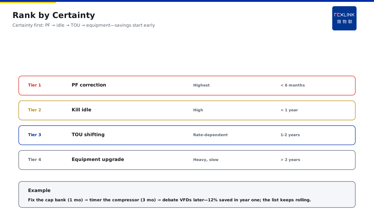
The principle — the high certainty first: the certainty = the predictable savings; The first — the reactive: the small, the fast and the highest; The second — the idle elimination: the timer and the auto — the high; The third — the peak shifting: the valley schedule and the storage — by the tariff; The fourth — the equipment upgrade: the VFD and the high-efficiency — the long.
In one sentence: the order by the certainty — the reactive → the idle → the peak → the equipment — the high first, the savings out.
The table:
| Rank | Opportunity | Certainty | Payback |
|---|---|---|---|
| 1 | Reactive | Highest | <0.5y |
| 2 | Idle | High | <1y |
| 3 | Peak | Medium | 1-2y |
| 4 | Equipment | Low | >2y |
The dynamic — the list not fixed: the re-rank after the data — the new waste in anytime — the rolling, the saving continuous. The output — by the rank: the rank/opportunity/investment/savings/payback/owner — one table, the divided. An example — The bank first (1 month) → the timer (3 months) → the VFD later — 12% of the first year. The logic is that the order decides "the first" — the certain and the short first — the rolling.
7. The Estimation and the Payback
The estimation — the baseline before vs the measured after: the difference the savings; The baseline — 2-4 weeks before: the weather, the output and the conditions; The payback — the investment / the annual value = the payback — one account each; The correction — the holidays, the maintenance and the fluctuation: the discount.
In one sentence: the savings = the baseline - the after; the payback = the investment / the annual — one each, the decision based.
The misconception — the rated power for the estimation: the actual lower — the measured, the honest. The output — one card each: the content/investment/savings/payback/risk — one card, all clear. An example — The timer 3,000 yuan — the 8,760 kWh × 0.8 = 7,008 yuan — the 5-month payback. The logic is that the savings "calculable" — the baseline and the measured, one account — the calculable, the owner pays.
8. The Rhythm (2 Weeks/3 Months)
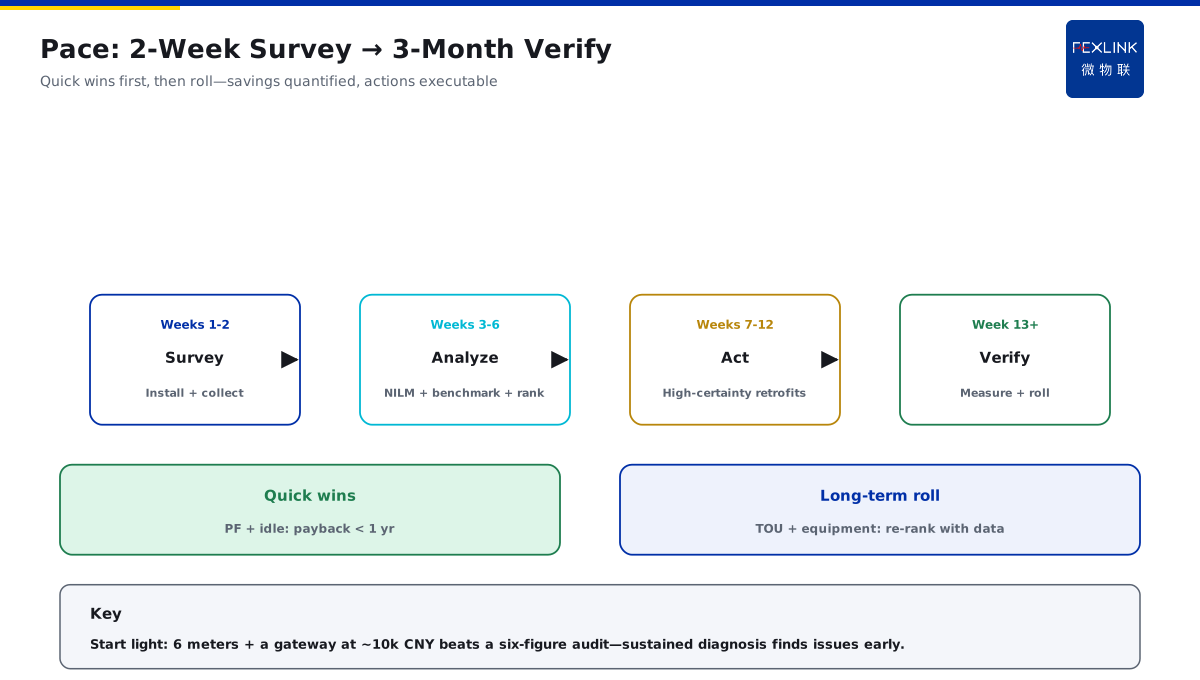
Step 1: the 2-week survey — the meters + the data + the list — the high-certainty located; Step 2: the 1-month pilot — the first rank — the savings verified; Step 3: the 3-month verification — the quarter comparison: the baseline vs the after — the savings settled; Step 4: the rolling — the verified promoted — the next batch.
In one sentence: the rhythm = the survey-pilot-verification-rolling — the 2-week list and the 3-month savings — the small steps, the rolling.
The table:
| Phase | Period | Action |
|---|---|---|
| Survey | 2w | The list |
| Pilot | 1m | The first |
| Verify | 3m | The settle |
| Roll | Rolling | The next |
The key — the deliverable each phase: the list, the data and the conclusion — the acceptance, the rhythm stable. The subjects — the plant energy + the platform + the service — three, the landing. The blockers — the data not 2 weeks: the baseline wrong; the pilot not verified: the savings doubtful — the prevented. An example — The 5 suggestions in 2 weeks → 3 in a month → the 9% in 3 months — the VFD next. The logic is that the rhythm is "the landing pace" — the small first and the verified first — the steady.
9. The Connection with the Energy-Carbon System
The direction — the diagnosis → the benchmarking → the carbon — one data line; The reuse — the diagnostic data → the benchmarking → the carbon activity — one set, three uses; The evolution — the diagnosis first, the benchmarking and the carbon last — the light to the heavy; The landing — the 4×3×2: the data-driven closed loop.
In one sentence: the diagnosis is "the entrance" — one set, three uses — the light to the heavy, the evolving.
The path — the first year the diagnosis: the base; the second the benchmarking: the normal; the third the carbon: the compliance — three years, three steps. The attention — the base unified: the same conversion coefficient — the unified, seamless. An example — The diagnostic data for the monthly benchmarking, the benchmarking for the annual carbon — one set, three uses. The logic is that the data "one collection, multi-use" — the shared base — the connection, the investment not wasted.
Back to the SFE/ESA/Tianyan family — the landing: the SFE for the power quality, the ESA for the sub-metering and the Tianyan C-01 for the reactive — from the data to the list, one line.
Scope and Limitations
- The conclusions in this article are intended for LV distribution and electrical-safety sites. Standard numbers (GB/T 17166, GB/T 13234) refer to their currently effective editions, and product parameters follow the latest FEXLINK selection handbook and product knowledge base.
- Quantitative criteria (protection zone, discharge and residual voltage, earth resistance, thresholds and grading) hold under the preconditions stated in this article. Where the site voltage level, earthing arrangement, environmental category or load profile differs, the figures must be recalculated. Specific configurations involving SFE power-quality controller, ESA all-element smart meter, Tianyan C-01(reactive-power compensation optimisation) should be verified against actual circuit parameters.
- Specific product models and parameters are subject to the latest selection handbook and product knowledge base; this article does not constitute selection or procurement advice.
- Standard numbers cited here refer to the currently effective editions; when a standard is revised, the related quantitative conclusions must be re-checked.
- Deployment and implementation for specific projects must be carried out by qualified engineers based on site survey and design drawings.
Frequently Asked Questions
A Practical Energy Audit Package for Small Factories
By the "key-circuit sub-metering + NILM load disaggregation + SEC benchmarking" light scheme — the reactive and the idle waste first