 FEXLINK Research Institute
The short answer
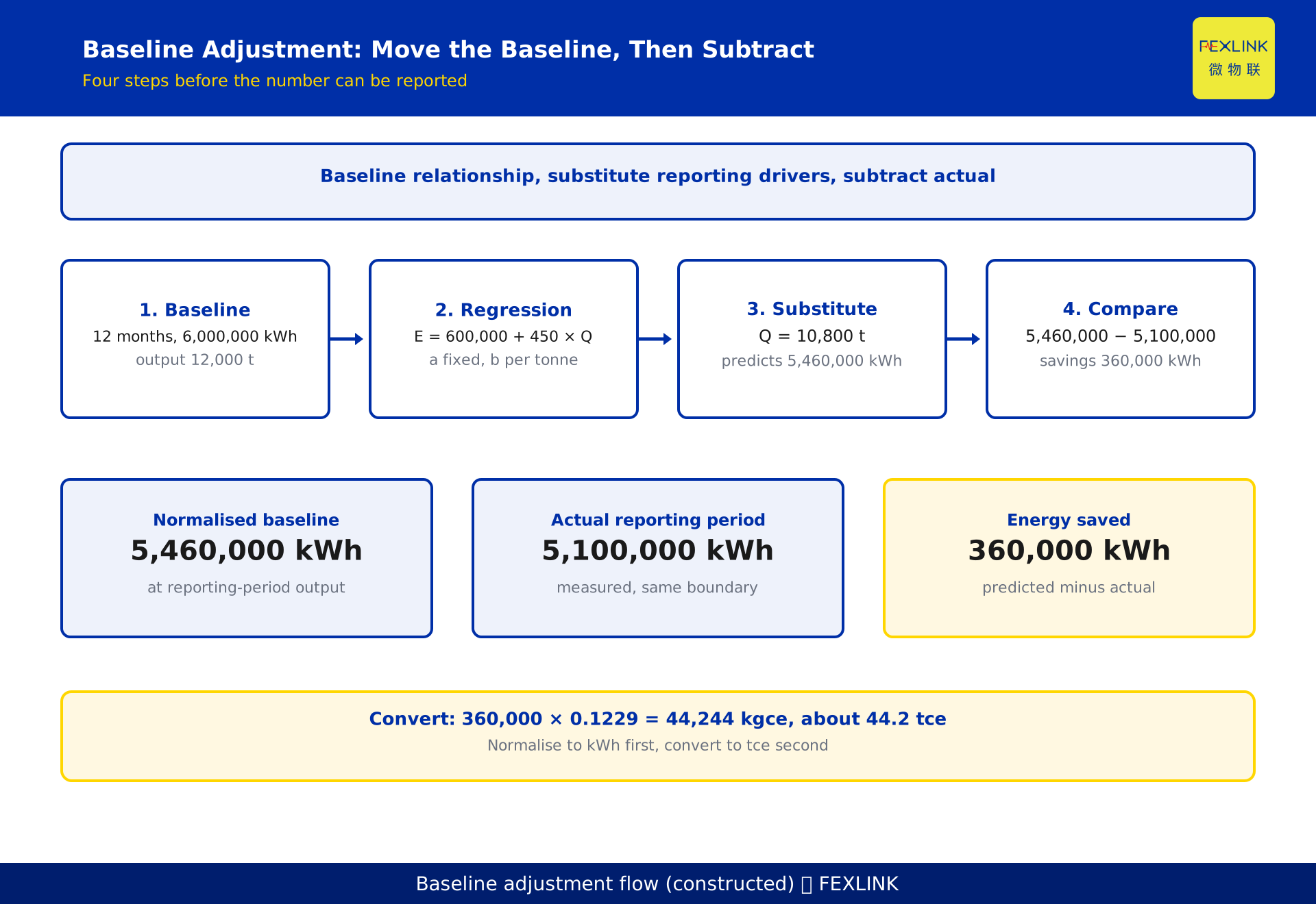
Energy savings are not "the meter reading after the retrofit minus the one before it". The calculation answers a counterfactual: how much energy would this period have used had the retrofit never happened? That figure comes from the baseline period's energy relationship — how output, weather and running hours drive consumption — and is reduced by what the reporting period actually used: savings = normalised baseline energy − actual reporting-period energy.
Until the two periods' conditions line up, the numbers are not comparable. Subtract them directly and what you get is savings plus the change in output, weather and operating pattern.
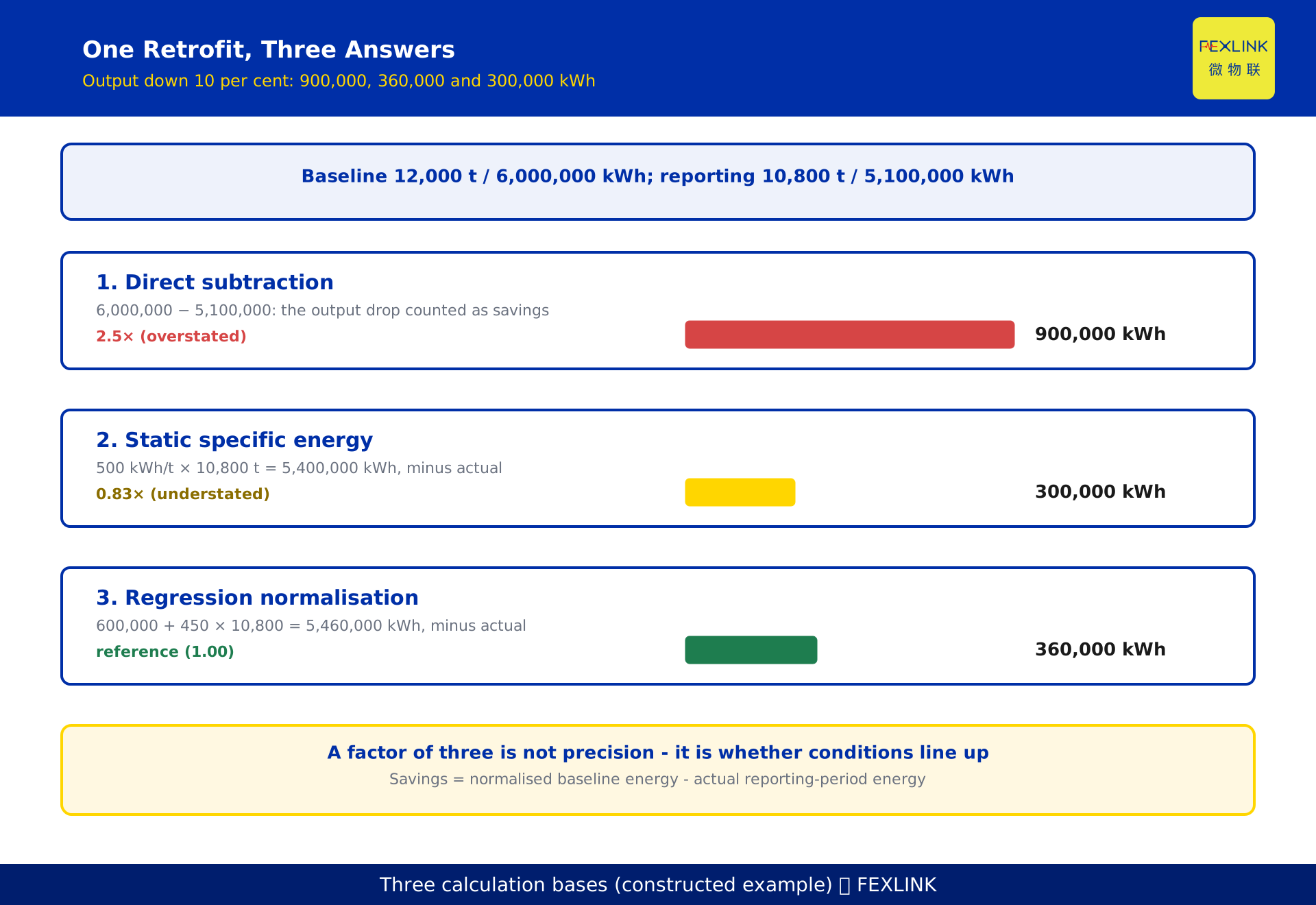
One retrofit, three methods, three answers: 900,000, 360,000 and 300,000 kWh. The difference is not precision but basis.
One retrofit, three answers
A constructed example, not a real client: a plant retrofits compressed air and fan motors. Baseline year: 12,000 t of output, 6,000,000 kWh. Year one after: 10,800 t, down 10 per cent, actual 5,100,000 kWh.
Direct subtraction: 6,000,000 − 5,100,000 = 900,000 kWh.
Static specific energy: 500 kWh/t × 10,800 t = 5,400,000 kWh, minus actual, 300,000 kWh.
Regression normalisation: E = 600,000 + 450 × Q, at Q = 10,800 t gives 5,460,000 kWh, minus actual, 360,000 kWh.
Output fell, so consumption was going to fall anyway; direct subtraction books all of that as savings. Static specific energy errs the other way: it assumes every kilowatt-hour scales with output, but 600,000 kWh here does not — standby, lighting, utilities. Spread over fewer tonnes, 60,000 kWh vanishes.
360,000 = 300,000 + 60,000. That addition is baseline adjustment: stripping the output change out and leaving only the energy not used at the same output.
Two national standards, two jobs
GB/T 13234-2018, *Determination of energy savings in organizations*, issued 17 September 2018, effective 1 April 2019. It supersedes GB/T 13234-2009, whose title read *Determination of energy savings in enterprises* — enterprises, not energy-using organisations — and adopts the core of ISO 50047:2016.
GB/T 28750-2012, *General technical rules for measurement and verification of energy savings*, covers something else: measurement and verification (M&V) — the measurement plan, data collection, calibration of baseline and reporting periods, verification of results. The two divide labour between method and measurement; neither replaces the other and the roles cannot be swapped. ASHRAE Guideline 14 adds what neither Chinese standard prescribes: statistical acceptance lines for a regression model.
Three words in one equation
Baseline energy is not what the baseline period consumed. 6,000,000 kWh is a fact, not a baseline. The baseline is the relationship between energy and its drivers — here E = 600,000 + 450 × Q — because it answers a counterfactual: at 10,800 t, what would an un-retrofitted plant have used?
Normalisation is not conversion to coal equivalent. Conversion changes the unit, from kWh to kgce; normalisation moves the baseline relationship onto the reporting period's drivers. Normalise first, still in kWh, then convert to tce.
Reporting-period energy must be measured on the same boundary. Move a line out of scope and consumption falls obligingly — but what fell is not savings.
Which drivers to adjust, and by which method
Output — physical tonnes, not output value; value contains price, and a price rise makes energy per unit of value fall without a joule saved. Weather — heating and cooling degree-days (HDD, CDD), which touch space heating, air conditioning and process cooling. Running hours — shifts, operating hours, units in service; drop from three shifts to two and part of the "saving" is equipment that never started. A driver belongs in the model when it correlates with baseline-period energy and actually changed in the reporting period.
A static baseline leaves the baseline specific energy unchanged: usable under 5 per cent output variation, but it distorts the moment output moves — 2.5× overstatement above. Specific-energy normalisation multiplies baseline specific energy by reporting output: fine for one product with a small fixed load, but the fixed load is diluted, understating by 60,000 kWh here. Multiple linear regression, E = a + b·Q + c·HDD + d·h, handles several drivers with continuous metering, at the cost of overfitting. Operating-mode stratification groups by product, shift or season and takes each group's mean.
Choose on three facts: output swing, fixed-load share, availability of sub-metering. Under 5 per cent swing with a small fixed load, static and regression land close; above 10 per cent, or fixed load over a tenth, use regression. If the boundary changed, rebuild the baseline.
Can the model be used? Three statistical tests
A fitted model is not yet usable. ASHRAE Guideline 14 sets acceptance lines by interval:
- Hourly: CVRMSE ≤ 30%, NMBE ≤ 10%.
- Monthly: CVRMSE ≤ 15%, NMBE ≤ 5%, R² ≥ 0.75.
The hourly line is 30 per cent, not 20 — the most miscopied figure in the field. Twenty per cent often gets written into a plan as a "more conservative" internal limit, but it is not the G14 hourly line; compliant models then get rejected and the project loops through acceptance.
CVRMSE measures the scatter of random error; NMBE measures systematic bias, which residuals do not cancel. Passing CVRMSE and failing NMBE means the predicted baseline sits high and savings come out inflated, and more data will not remove the bias. R² cannot stand in for either: over a wide range it can exceed 0.9 while prediction error still breaches the line.
Uncertainty: savings come with a ±
Savings are calculated; every input carries error, so savings do too. Three sources: measurement (meter accuracy class, transformer error, reading time not aligned with the accounting period), model (CVRMSE, whether the baseline year was typical), drivers (output ledger, weather data, running-hour records). Combine in quadrature by common practice; formal evaluation follows general metrology rules.
Scale: 5,100,000 kWh at ±0.5 per cent meter error is ±25,500 kWh; a CVRMSE of 12 per cent against a predicted 5,460,000 kWh is about ±655,200 kWh. The model term exceeds the 360,000 kWh of savings. Combined roughly, savings sit between −295,000 and 1,015,000 kWh (360,000 ± 655,000) — and the interval crosses zero.
Crossing zero means one year of data cannot yet show that energy was saved. Do not bury the interval; extend the reporting period, add sub-metering, refine the model. Treating CVRMSE as prediction error is an order-of-magnitude conversion, not a formal evaluation, but it makes the point: savings reported without an interval are not reported. No standard sets a threshold of "uncertainty under some percentage of savings".
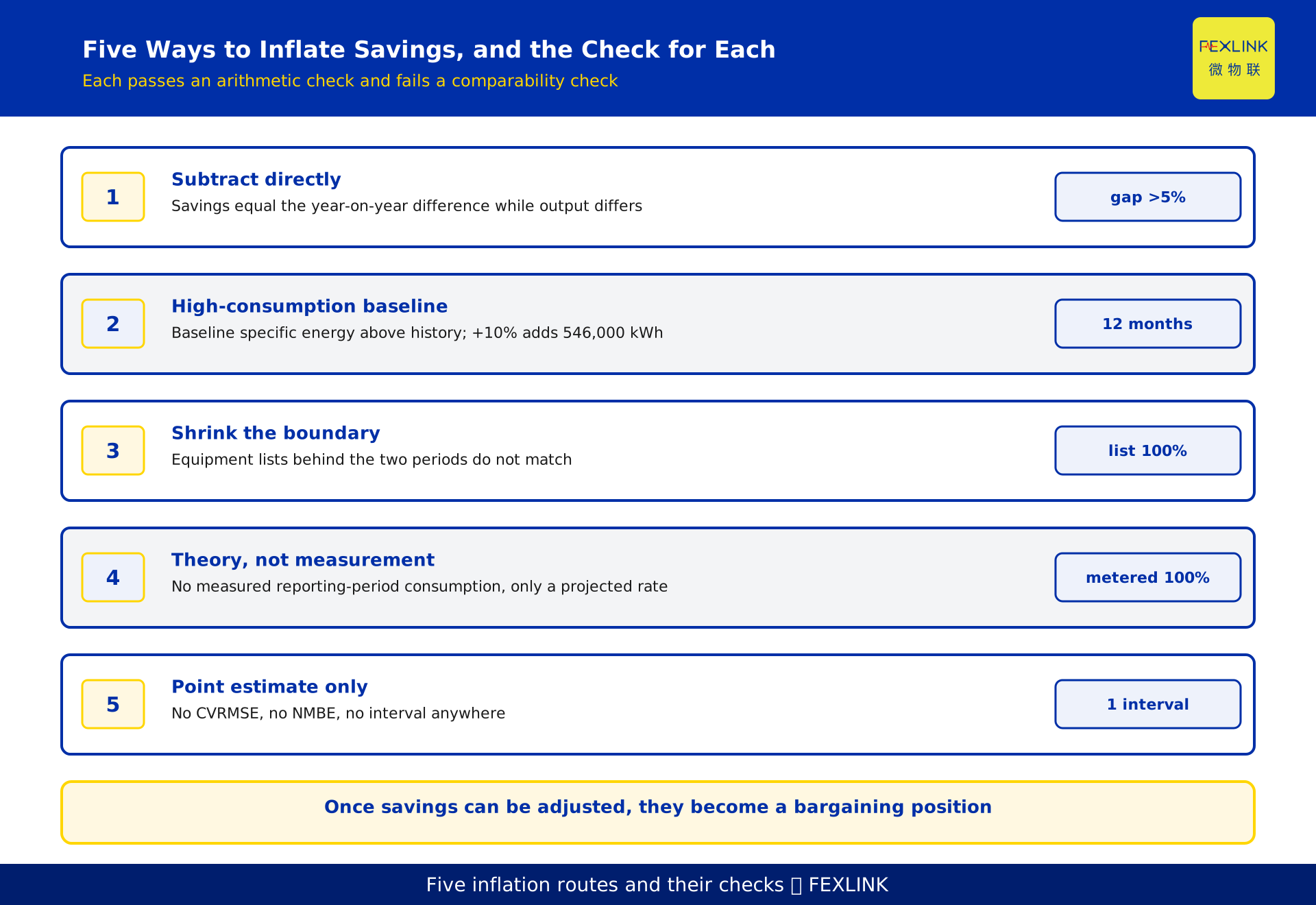
Five ways to inflate savings
One: subtract directly. Two totals, one subtraction. Tell-tale: savings equal the year-on-year difference exactly while output differs.
Two: pick a high-consumption baseline. Choose an expensive year or month. Tell-tale: baseline specific energy sits above the historical average; lift the baseline 10 per cent and savings here inflate by 546,000 kWh.
Three: shrink the boundary. Move a workshop or line out of scope. Tell-tale: the equipment lists behind the two periods do not match.
Four: theory instead of measurement. Nameplate efficiency, catalogue data, a supplier's promise. Tell-tale: no measured reporting-period consumption, only a projected saving rate.
Five: report a point estimate only. A single 360,000 kWh, no interval, no model criteria. Tell-tale: no CVRMSE, no NMBE.
None of the five survives a comparability check. Once savings can be adjusted, they stop being a performance indicator and become a bargaining position.
A constructed example, worked end to end
Constructed; not a real client.
Baseline: twelve pre-retrofit months — 12,000 t, 6,000,000 kWh, 500 kWh/t. Model: E = a + b × Q gives a = 600,000 kWh and b = 450 kWh/t; back-substituting, 600,000 + 450 × 12,000 = 6,000,000 kWh, matching measurement. Compare: at 10,800 t, normalised baseline 600,000 + 450 × 10,800 = 5,460,000 kWh against actual 5,100,000 kWh, savings 360,000 kWh. Convert: 360,000 × 0.1229 = 44,244 kgce ≈ 44.2 tce.
| Method | Baseline energy | Savings | Relative to regression |
|---|---|---|---|
| Direct subtraction | 6,000,000 kWh | 900,000 kWh | 2.5× (overstated) |
| Static specific energy | 5,400,000 kWh | 300,000 kWh | 0.83× (understated) |
| Regression normalisation | 5,460,000 kWh | 360,000 kWh | 1.00 (reference) |
The 900,000 kWh converts to 110,610 kgce ≈ 110.6 tce, 66.4 tce above the regression answer. Those 66.4 tce came from the 10 per cent output drop, not from the retrofit: less work done, not less energy per unit of work.
Interval: −295,000 to 1,015,000 kWh, crossing zero, so one year cannot show that savings occurred. Remedies: a 24-month reporting period, separate metering for compressed air and fans, running hours in the model.
Savings are not one subtraction but a chain from baseline to reporting period, from model to interval; loosen any link and the final number stops being credible.
Making adjustment routine
Fix the M&V plan before the retrofit. Afterwards is marking your own exam. Five items in writing: boundary, baseline period with exclusions, driver list, model form, acceptance criteria. This is where an energy performance improvement system starts.
Sub-meter the drivers. Sub-circuit energy is the dependent variable; output, weather and running hours are the drivers. Estimate any one and the model is soft. Sub-circuits can be metered with the FEXLINK ESA full-parameter smart meter (ESA-22111-R to ESA-22161-R, six current ratings, 3×220/380V, RS485 Modbus), read on a fixed cycle and archived. The meter answers where the dependent variable comes from; the drivers still depend on ledgers and records. Where baseline data are thin, run an energy diagnosis first: complete the sub-metering, align the ledgers.
Fix the model in the platform. The TIANYAN E module (energy analysis) stores the baseline regression, substitutes each month's drivers and outputs the normalised baseline and deviation, so every month shows the savings and the interval width. Cover at least one full production cycle, and a full year where seasonality matters.
FAQ
Q: Savings or percentage savings — which do we report?
Both, with the denominator stated. Savings are absolute, in kWh or tce. A percentage needs a denominator — baseline energy, or the energy implied by baseline output — and without it, "15 per cent saved" can mean three things.
Q: Output rose and the calculated savings are negative. Is that normal?
Yes, and usually it is the honest answer. A negative result after normalisation means energy per unit of output rose: the retrofit underdelivered, or operating practice deteriorated, or equipment aged. Investigate the cause; do not tune the model until the sign flips.
Q: Can we just use the fall in specific energy per unit of product?
Only where the fixed load is small. In the example the fixed load is 10 per cent and output fell 10 per cent, so the method understates by 60,000 kWh. The test: fixed load under 5 per cent and output swing under 5 per cent; exceed either and use regression.
Q: Equivalent value or equal value for electricity?
Follow the reporting system and the contract, but keep one basis across the table and across years. The equivalent value is a hard 0.1229 kgce/kWh. The equal value uses the previous year's national thermal-power supply coal rate, roughly 0.30–0.31 kgce/kWh. Natural gas is roughly 1.1–1.3 kgce/m³, steam roughly 0.09–0.12 kgce/kg, and working media must be counted.
Q: A third-party assessment differs sharply from our figure. What do we compare first?
Four things, in order: whether the boundary is the same meters and equipment; whether the baseline period and exclusion rules match; whether the driver list and model form match; whether the acceptance criteria match. If they differ, the gap is not "who calculated it wrong" but "not the same calculation".
Scope and limitations
- This article follows GB/T 13234-2018, *Determination of energy savings in organizations* (issued 17 September 2018, effective 1 April 2019, superseding GB/T 13234-2009 *Determination of energy savings in enterprises* and adopting the core of ISO 50047:2016) and GB/T 28750-2012, *General technical rules for measurement and verification of energy savings*. Clause text follows the edition in force; no clause numbers are cited.
- ASHRAE Guideline 14 acceptance lines: hourly CVRMSE ≤ 30 per cent and NMBE ≤ 10 per cent; monthly CVRMSE ≤ 15 per cent, NMBE ≤ 5 per cent, R² ≥ 0.75.
- Conversion factors move with year, gas quality and steam parameters: electricity at the equivalent value is a hard 0.1229 kgce/kWh; the equal value uses the previous year's national thermal-power supply coal rate (roughly 0.30–0.31 kgce/kWh); natural gas roughly 1.1–1.3 kgce/m³; steam roughly 0.09–0.12 kgce/kg; working media must be counted. Magnitudes only.
- The figures in sections one and eight are constructed and do not represent any real client; the 12 per cent CVRMSE is assumed.
- This article covers how savings are calculated from a baseline. It does not cover how a baseline is established, which belongs to KD-0422.
- Carbon reductions are outside scope. ESA smart-meter range, parameters and interfaces follow the current selection manual; range, circuit count and supply method are customizable. TIANYAN E functions follow the current release.
Frequently Asked Questions
Savings or percentage savings — which do we report?
Both, with the denominator stated. Savings are absolute, in kWh or tce. A percentage needs a denominator — baseline energy, or the energy implied by baseline output — and without it, "15 per cent saved" can mean three things.
Output rose and the calculated savings are negative. Is that normal?
Yes, and usually it is the honest answer. A negative result after normalisation means energy per unit of output rose: the retrofit underdelivered, or operating practice deteriorated, or equipment aged. Investigate the cause; do not tune the model until the sign flips.
Can we just use the fall in specific energy per unit of product?
Only where the fixed load is small. In the example the fixed load is 10 per cent and output fell 10 per cent, so the method understates by 60,000 kWh. The test: fixed load under 5 per cent and output swing under 5 per cent; exceed either and use regression.
Equivalent value or equal value for electricity?
Follow the reporting system and the contract, but keep one basis across the table and across years. The equivalent value is a hard 0.1229 kgce/kWh. The equal value uses the previous year's national thermal-power supply coal rate, roughly 0.30–0.31 kgce/kWh. Natural gas is roughly 1.1–1.3 kgce/m³, steam roughly 0.09–0.12 kgce/kg, and working media must be counted.
A third-party assessment differs sharply from our figure. What do we compare first?
Four things, in order: whether the boundary is the same meters and equipment; whether the baseline period and exclusion rules match; whether the driver list and model form match; whether the acceptance criteria match. If they differ, the gap is not "who calculated it wrong" but "not the same calculation".