 FEXLINK Research Institute
Direct Answer
How exactly do you build an energy baseline? An energy baseline is commonly built with a regression model: energy is the dependent variable and production, degree days and shifts are the independent variables (for example, E = a + b x production + c x degree days); after the retrofit, use the same model to predict the "energy that should have been consumed" and compare it with the actual to obtain the true saving.
A scenario: A factory wants to build an energy baseline — but it only knows how to compute a historical average — when production changes, the average becomes distorted. The logic is that an average baseline assumes "energy is constant", while a regression baseline assumes "energy follows the variables" — with regression normalization using production and temperature, the energy prediction keeps up with the business.
1. Why an Average Baseline Is Distorted
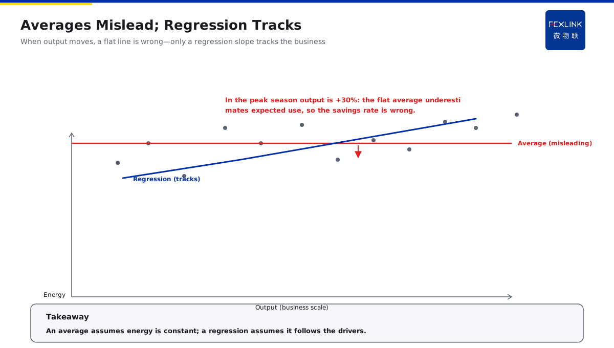
The problem of the average — the static assumption: the average assumes energy is constant and fails once the business changes; The error of the average — the production effect: when production doubles, the average clearly underestimates the "energy that should have been consumed"; The bias of the average — the temperature effect: with high air-conditioning load in summer, the average cannot reflect seasonal differences; The conclusion of the average — a distorted saving rate: after the retrofit meets a high-production season, the saving rate is understated or inflated.
In one sentence: an average baseline is a static assumption — it fails once production and temperature change — only a regression model keeps up with the business.
The comparison table of the average and the regression:
| Comparison dimension | Average baseline | Regression baseline |
|---|---|---|
| Assumption | Energy is constant | Energy follows variables |
| Response to production change | None | Responds by the slope |
| Response to temperature change | None | Responds by the coefficient |
| Adaptation to business fluctuation | Poor | Good |
| Credibility of the saving rate | Low | High |
An example: A factory uses an average baseline: it uses the monthly average energy of the whole year — after the retrofit meets the peak season with production +30% — the saving rate computed by the average is clearly distorted. The logic is that the average folds months of different production and temperature into one number — when the business fluctuates heavily, the average is neither the level "that should have been" of the high-production month nor the level of the low-production month — a regression model predicts with the variable relationship and keeps up with the business.
2. The Form of a One-Variable Regression Baseline Model
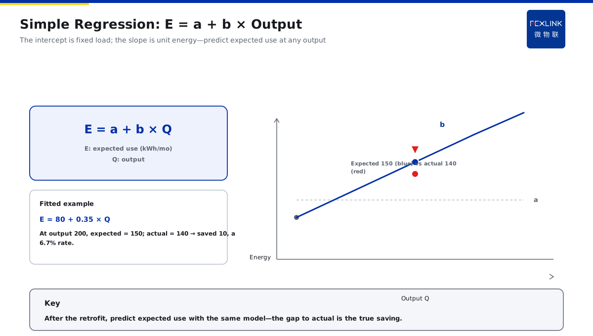
The form of the model — E = a + b x production: energy (E) changes linearly with production; The intercept a — fixed energy: the base energy that does not change with production (lighting, office, etc.); The slope b — unit energy: the incremental energy per unit of production; The meaning of the fit — normalization: the model gives the "energy that should have been consumed" at any production level.
In one sentence: one-variable regression E = a + b x production — the intercept is fixed energy and the slope is unit energy — the model predicts the should-be energy at any production level.
An example: A factory fits: E = 80 + 0.35 x production (10,000 kWh/month, production in 10,000 tons) — when the monthly production is 2 million tons, the predicted should-be energy = 80 + 0.35 x 200 = 1.5 million kWh. The logic is that the regression quantifies the production-energy relationship — when production is 200, the should-be is 150; when production is 250, the should-be is 167.5 — after the retrofit the actual is 140, compared with the predicted 150, the saving is 100,000 kWh — the saving rate is 6.7%.
3. Multiple Regression: Modeling Production, Temperature and Shifts Together
The form of the multiple model — E = a + b x production + c x degree days + d x shifts: several variables explain energy together; The production variable — business scale: the higher the production, the higher the energy (equipment follows); The temperature variable — seasonal load: degree days (HDD/CDD) quantify heating and cooling load; The shift variable — running hours: more shifts mean longer running and higher energy.
In one sentence: multiple regression models production, temperature and shifts together — energy changes are explained more completely.
The calculation scope of degree days — cooling degree days (CDD) is the sum of positive differences between the daily average temperature and a base temperature (often 26°C); heating degree days (HDD) is the sum of positive differences between a base temperature (often 18°C) and the daily average temperature — the higher the degree days, the heavier the heating and cooling load and the higher the energy.
An example: A factory fits a multiple model: E = 50 + 0.30 x production + 2.5 x CDD + 12 x shifts — in a month with production of 1.8 million tons, CDD of 20 and 2 shifts — the predicted should-be energy = 50 + 54 + 50 + 24 = 1.78 million kWh. The logic is that a one-variable model explains only production and misses temperature and shifts — the multiple model includes all three main drivers — the prediction error is smaller and the saving rate is more credible — the more variables, the closer the model is to the real energy structure.
4. How to Select Independent Variables
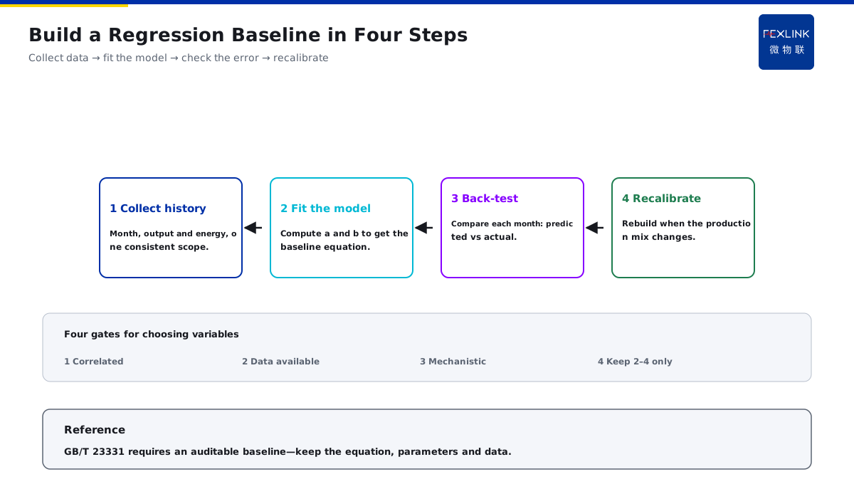
Principle one, correlation — check correlation first: only variables significantly correlated with energy enter; Principle two, availability — data can be obtained: the variable must have a stable historical data source; Principle three, interpretability — clear mechanism: the relationship between the variable and energy has physical logic; Principle four, few and precise — control the number: 2-4 variables are appropriate to avoid overfitting.
In one sentence: variable selection is correlation, availability, interpretability and few-but-precise.
The comparison table of independent variables:
| Variable | Quantification scope | Effect mechanism | Suggestion |
|---|---|---|---|
| Production | Output/output value | Energy-using equipment follows production | Must |
| Temperature | Degree days HDD/CDD | Heating and cooling load changes with temperature | Suggested |
| Shifts | Running hours/shift count | Running time affects energy | Depending on the case |
| Weather sun/rain | Rainy days | Affects auxiliary load | Optional |
An example: A factory selects variables: it checks correlation first — the correlation between production and energy is 0.9 and that between temperature and energy is 0.6 — it keeps production and temperature and removes weakly correlated variables. The logic is that variable selection is not the more the better — weakly correlated variables with unclear mechanisms introduce noise — production and temperature are the main drivers, so select these two first — add shifts when needed — with few and precise variables, the model is stable and interpretable.
5. Model Fit Quality and the Data Period
Fit quality — the R² indicator: the closer R² is to 1, the stronger the explanatory power; The R² reference — the empirical threshold: an energy baseline generally requires R² above 0.7; The data period — coverage: take 12-24 months of data covering complete seasons and production ranges; Outlier removal — data cleaning: remove months with maintenance, shutdown and abnormal events.
In one sentence: fit quality is judged by R² (0.7 or above is good) — take 12-24 months of data covering complete seasons and remove outliers.
The interpretation reference of R² — R² above 0.9: the model has very strong explanatory power and small prediction error; R² between 0.7 and 0.9: the model is usable for routine saving accounting; R² below 0.7: the explanatory power is insufficient and variables or data need adjustment.
An example: A factory validates: the model R² is 0.85 — the data covers 18 months including winter and summer — the model passes. The logic is that a low R² means the model has not explained enough — a key variable may be missing or the data contains outliers — add variables and clean the data first, then refit — when the data period covers complete seasons, the model does not fail in extreme-weather months.
6. How to Predict the Baseline Energy After the Retrofit
The logic of prediction — the same model: use the same regression model after the retrofit to predict the "energy that should have been consumed"; Input current variables — current production and temperature: input the monthly production and degree days into the model; Compare with the actual — the true saving: predicted should-be energy − measured energy = the saving; Consistent scope — variable scope: prediction and actual use the same production and temperature scope.
In one sentence: predicting after the retrofit = the same model + current production and temperature input → should-be energy, compared with the measured to obtain the true saving.
An example: A factory after the retrofit: the monthly production is 2 million tons and CDD is 15 — the model predicts a should-be energy of 1.65 million kWh — the measured is 1.5 million kWh — the saving is 150,000 kWh and the saving rate is 9.1%. The logic is that the key of prediction is "the same model and the same scope" — the model built before the retrofit continues to be used after — input the actual monthly production and temperature to predict "what would have been consumed without the retrofit" — the difference from the measured is the retrofit contribution — the saving result stands up to review.
7. The Practical Flow and Common Pitfalls
Flow one, collect data — collect historical energy, production and temperature data; Flow two, clean — remove maintenance, shutdown and abnormal months; Flow three, fit — fit the model with a regression tool and check R²; Flow four, validate — verify the prediction error with held-out data; Flow five, use — predict the should-be energy monthly after the retrofit and compute the saving rate.
In one sentence: the practical flow is data collection, cleaning, fitting, validation and use.
The four common pitfalls — pitfall one: using the average directly as the baseline; pitfall two: an incomplete data period of only half a year; pitfall three: missing the temperature variable so the summer prediction fails; pitfall four: changing the statistical scope after the retrofit so before and after are incomparable.
Back to the TIANYAN product match — the TIANYAN engine E module (energy analysis) has built-in regression modeling: it automatically takes historical energy, production and temperature data and fits E = a + b x production + c x degree days — after the retrofit it automatically predicts the monthly should-be energy and computes the saving rate — the model parameters and data are fully archived and re-checkable.
An energy baseline quantifies the energy-variable relationship with regression — E = a + b x production + c x degree days — after the retrofit, the same model predicts the should-be energy and the comparison with the measured gives the true saving — the era of the average is over, and regression normalization is the foundation of credible saving results.
Scope and Limitations
- The conclusions in this article are intended for LV distribution and electrical-safety sites. Standard numbers (GB/T 23331, GB/T 13234) refer to their currently effective editions, and product parameters follow the latest FEXLINK selection handbook and product knowledge base.
- Quantitative criteria (protection zone, discharge and residual voltage, earth resistance, thresholds and grading) hold under the preconditions stated in this article. Where the site voltage level, earthing arrangement, environmental category or load profile differs, the figures must be recalculated. Specific configurations involving Tianyan engine, E track (energy analytics) should be verified against actual circuit parameters.
- Specific product models and parameters are subject to the latest selection handbook and product knowledge base; this article does not constitute selection or procurement advice.
- Standard numbers cited here refer to the currently effective editions; when a standard is revised, the related quantitative conclusions must be re-checked.
- Deployment and implementation for specific projects must be carried out by qualified engineers based on site survey and design drawings.
Frequently Asked Questions
How Exactly Do You Build an Energy Baseline
An energy baseline is commonly built with a regression model: energy is the dependent variable and production