 FEXLINK Research Institute
The short answer
Power factor is one division: cosφ = active power ÷ apparent power. It does not change how much useful work you get; it decides how much the network must deliver for it. At 0.90 every 100 kW draws 111.1 kVA; at 0.95 it draws 105.3 kVA. The 5.8 kVA gap is extra current, loss and capacity.
The difference lands in three places: the tariff adjustment (credit above the local assessment value, surcharge below — direction certain, size set by the local document in force), line loss (inverse to cos²φ, about 10.3% lower) and capacity (down 5.3%). For 800 kW the move needs about 124 kvar. Whether it pays back fast depends on whether the local adjustment is really applied.
1. Decoding the reading: one division
The 0.9 on the meter is a division: cosφ = P / S. Apparent power S is voltage times current (√3·U·I in three-phase); active power P does the real work; the difference is reactive power Q, with S² = P² + Q².
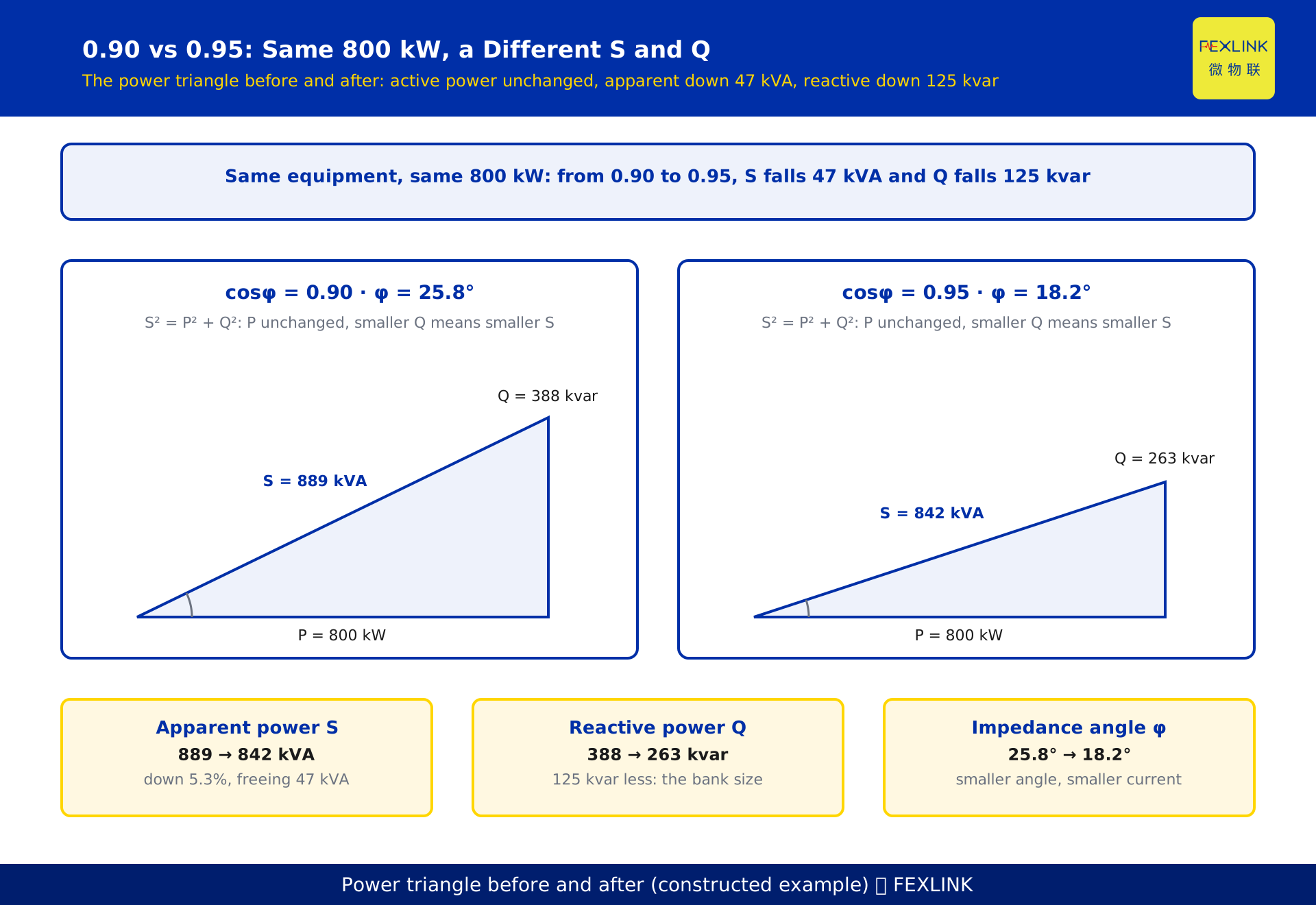
Put another way: current is set by apparent power, not by active power. Delivering 800 kW at 0.90 makes the line carry 889 kVA; at 0.95, 842 kVA. Current falls 5.3%, heating follows current squared, and line loss falls about 10%.
Three reading habits. Read P and Q together: at night cosφ may sit at 0.6 while absolute reactive power is tiny; at full load, 0.88 with a large Q is the real problem. Know whether you read a total or a phase: with imbalance the total hides the weakest phase. Watch the period: the adjustment uses billing-cycle energy, not an instant.
2. Which number is on the meter: displacement or total power factor
Displacement power factor (DPF), or fundamental power factor, counts only the 50 Hz fundamental — that is cosφ₁.
Total power factor (PF) includes harmonics: PF = P/S, where S contains distortion power.
With harmonics PF is lower than DPF. A common approximation is PF ≈ DPF / √(1 + THD²ᵢ), where THDᵢ is current total harmonic distortion, valid only when voltage distortion is negligible.
Why it matters: capacitors compensate fundamental reactive power, not harmonics. If the meter shows PF 0.88 while DPF is 0.93, the gap is harmonic; capacitors will not close it and may amplify harmonics until they fail. The answer is harmonic mitigation.
Which number the utility assesses is governed by the local grid company's metering rules; confirm it before installation.
3. 0.90, 0.95, 0.99: the difference is in what gets shipped
Per 100 kW of active power.
| cosφ | tanφ | Apparent power S (kVA) | Reactive Q (kvar) | Loss index 1/cos²φ |
|---|---|---|---|---|
| 0.90 | 0.484 | 111.1 | 48.4 | 1.235 |
| 0.95 | 0.329 | 105.3 | 32.9 | 1.108 |
| 0.99 | 0.142 | 101.0 | 14.2 | 1.020 |
| 1.00 | 0 | 100.0 | 0 | 1.000 |
Returns diminish. 0.90 to 0.95 saves 5.8 kVA per 100 kW; 0.95 to 0.99 another 4.3 kVA; 0.99 to 1.00 only 1.0 kVA.
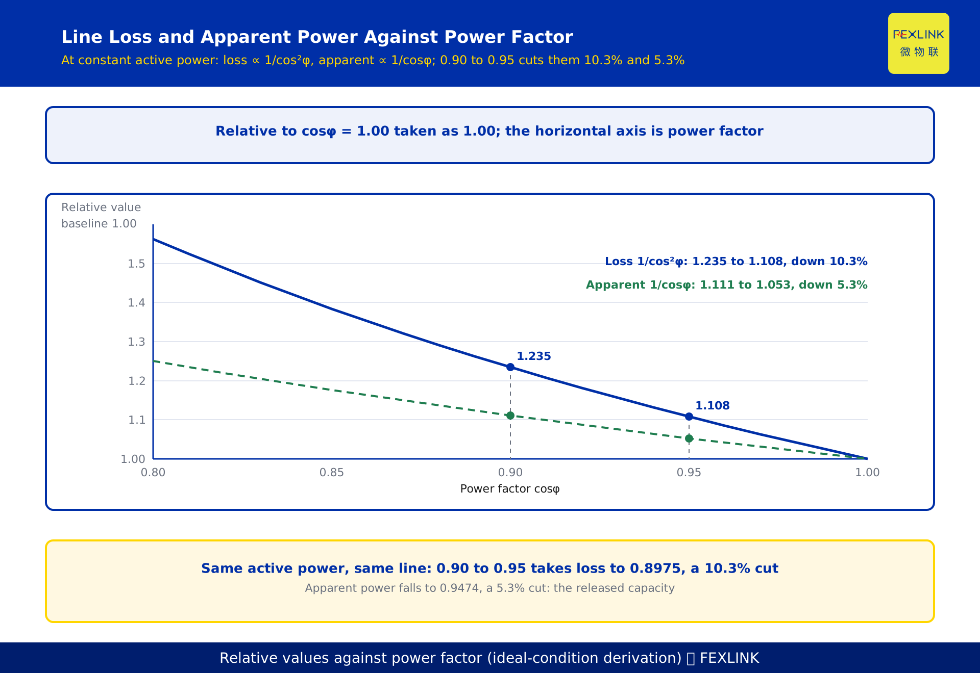
The marginal loss benefit is larger at low power factor. Loss falls 10.3% from 0.90 to 0.95 but only 7.9% from 0.95 to 0.99. A poor power factor gains most from the first bank; at 0.95 the next step may not pay for itself.
0.99 is not the target. At 0.99 there is almost no reactive margin, so any drop in load causes overcompensation: reverse reactive flow, voltage rise, switching oscillation. The target belongs near 0.95 — above the assessment value, with margin for load swings.
4. The tariff adjustment: tiered by design, percentages by local document
Most bills carry a power-factor tariff adjustment line: fix an assessment value, compute the billing-cycle average power factor, compare, then apply a tiered credit or surcharge.
The assessment value is not a nationwide 0.9. The common figure is 0.9, but some classes are assessed at 0.85 or 0.80 — check the local document. 0.9 is a tariff benchmark, not a mandatory equipment standard: no Chinese national standard requires it.
The ratios are tiered, non-linear and local. Above the assessment value you get a tiered credit; below it, a surcharge that grows with the shortfall and is usually capped. The specific tiers and percentages follow the local grid company's current power-factor tariff rules or supply regulations. No tier table is printed here: practice differs by province and policy changes, so copying an old table is worse than having none.
So do not memorise ratios: pull the last three bills, see whether that line is positive or negative, then look up the tier table in force.
Section 8 uses a hypothetical 0.1% credit per 0.01 to show the magnitude — a tidy number to demonstrate the arithmetic, not any jurisdiction's standard; real ratios must come from the local document.
5. Line loss: inversely proportional to the square of power factor
In a three-phase circuit I = P / (√3 · U · cosφ) and line loss is 3I²R. Substituting I:
Loss = 3R · P² / (3U²·cos²φ) = R·P² / (U²·cos²φ)
With the same active power, voltage and conductor resistance, line loss is inversely proportional to cos²φ. Raising cosφ from 0.90 to 0.95 turns the loss into (0.90/0.95)² = 0.9474² = 0.8975 of its former value — a 10.3% reduction.
That is a ratio, not a quantity. A 20.0 kW loss becomes 17.95 kW, saving 2.05 kW per hour, about 16,400 kWh over 8,000 hours; a 5 kW loss saves only 0.5 kW. Measure the loss base first.
Copper loss behaves the same way; iron loss does not. So the system-wide reduction depends on the split and will not be 10.3% everywhere.
One caveat: the derivation assumes constant active power; compensation raises the busbar voltage slightly and the load may draw more, so verify by measurement.
6. Capacity released: 5.3% less transformer for the same active power
S = P / cosφ. At 0.90, S = 1.111P; at 0.95, S = 1.053P. The ratio 0.90/0.95 = 0.9474, so apparent power falls 5.3%. For 800 kW that is 889 kVA down to 842 kVA, freeing 47 kVA.
Those 47 kVA become money or margin where a capacity charge is billed on maximum demand in kVA, where a transformer near full load defers an upgrade, or where a thermally tight feeder gains headroom.
The value depends on using the margin: a transformer at 40% load frees 47 kVA on paper only — leave it out of the payback.
7. Sizing the compensation: one subtraction
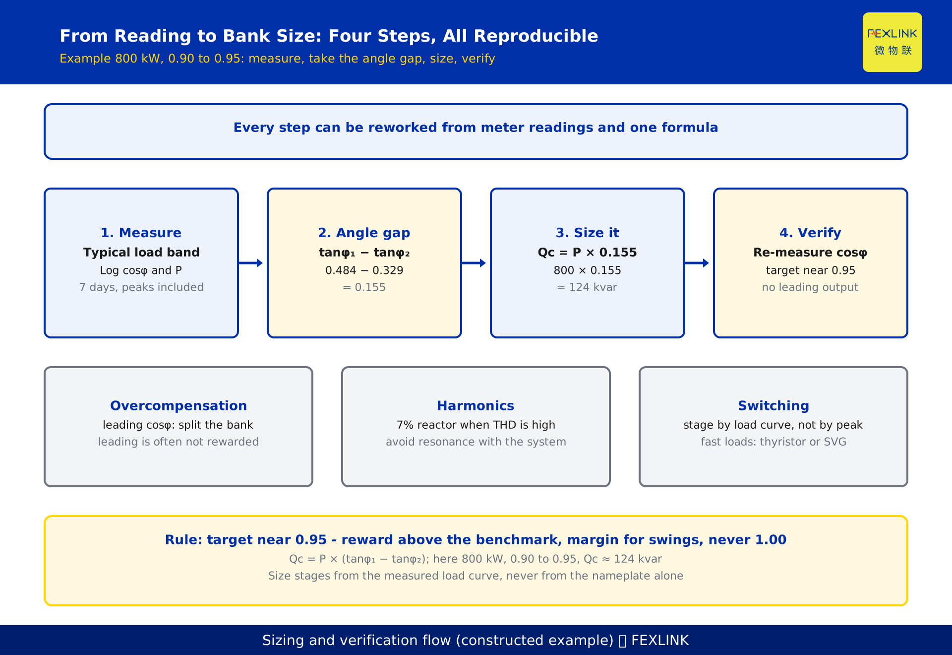
Qc = P × (tanφ₁ − tanφ₂), where φ₁ is the angle before compensation and φ₂ the target. Since Q = P·tanφ, the drop from P·tanφ₁ to P·tanφ₂ is what must be supplied locally.
For 800 kW, 0.90 to 0.95: tanφ₁ = 0.484, tanφ₂ = 0.329, difference 0.155, so Qc = 800 × 0.155 ≈ 124 kvar. The unrounded 0.1556 gives 124.5 kvar; a 125 kvar bank is the usual practical choice.
Three corrections. Capacitor output varies with voltage squared: a 400 V capacitor on a 380 V bus delivers only (380/400)² ≈ 0.90 of rating, so size against actual bus voltage. Do not fit for peak load in one step: a fixed bank overcompensates at 30% load, so split into 3–5 switched stages and hold cosφ between 0.92 and 0.97. Use reactors with harmonics: a capacitor resonates with system inductance and amplifies harmonic current until it fails; a 7% reactor commonly suppresses the 5th harmonic and above, chosen from measured orders.
8. A worked example: the arithmetic for 800 kW
Every price, ratio and hour below is hypothetical, chosen to demonstrate the arithmetic. None represents a current tariff or any supplier's quotation.
Assumptions: 800 kW constant, 8,000 hours a year, 0.70 CNY/kWh; cosφ from 0.90 to 0.95; line loss 20.0 kW before compensation; installed cost 200 CNY/kvar; monthly bill 500,000 CNY; hypothetical credit 0.1% per 0.01.
| Benefit | Arithmetic | Annual value |
|---|---|---|
| Lower line loss | (20.0 − 17.95) kW × 8,000 h × 0.70 CNY | about 11,500 CNY |
| Tariff credit | 0.5% × 500,000 CNY/month × 12 | about 30,000 CNY |
| Capacity released | 47 kVA × hypothetical 30 CNY/kVA·month × 12 | about 17,000 CNY |
| Total | about 58,500 CNY |
Investment 124 kvar × 200 CNY/kvar ≈ 25,000 CNY. Simple payback ≈ 25,000 ÷ 58,500 ≈ 0.43 years, about five months.
Sensitivity matters more than the headline: at half the ratio, payback is 0.57 years; with a capacity-based charge, 0.60 years; with no adjustment, only the 11,500 CNY loss benefit remains and payback stretches to 2.2 years — worthwhile, but not fast.
Hence the conditional conclusion: fast payback depends on whether the local adjustment is really applied, and on whether your load curve makes the released capacity useful.
9. Choosing the target and three checks
Aim for 0.95, not 1.00. The assessment value is usually 0.9, so 0.95 sits in the upper tier, with 0.03–0.05 of margin for load swings.
Check one, overcompensation. If cosφ goes leading after switching, you have fitted too much: reactive power flows back, voltage rises, capacitor and transformer losses increase, and some local rules do not reward a leading power factor. Reduce or split the bank.
Check two, harmonics. Measure before and after switching. A sharply rising harmonic current means resonance: you need reactors or a filtered bank.
Check three, switching. Contactor inrush can reach dozens of times rated current and frequent switching shortens life; for welders, rolling mills and lift banks, thyristor switching or a static var generator fits.
The SFE power-quality controller captures per-phase voltage, current, active and reactive power, power factor and harmonics, archiving before-and-after curves; stage sizing can run through Tianyan C-01 reactive-power compensation optimisation from the measured load curve. The same data shows whether the problem is capacitance or harmonics.
FAQ
Q: How much will I save going from 0.90 to 0.95 in a year?
Three sources: the tariff credit, lower line loss and released capacity, all local-dependent. Only the direction is certain; the amount must come from your own bills and load curve.
Q: Where do I find the credit and surcharge table?
The local grid company's current rules; the annexes to your supply contract; your own bill, where the adjustment line lets you back out the ratio. Do not use an old table from the internet — version and region are likely wrong.
Q: If there is a reward, why not compensate to 1.00?
1.00 is physically unreachable and commercially unattractive: returns diminish, overcompensation risk rises sharply, and finer staging costs more. 0.95 balances benefit against risk.
Q: The meter says 0.95 but the bill says 0.91. Which is wrong?
Probably neither. Four differences: location (meter in the workshop, assessment at the gateway, with transformer and feeder losses between), period (instantaneous against an energy average), method (PF with harmonics against the fundamental), averaging (energy-weighted, not an arithmetic mean).
Q: The capacitor bank is in but the power factor barely moved. Why?
In order of likelihood: capacitors failed > switching circuit not operating > stages too small > busbar voltage low > harmonics cutting capacity. Measure capacitor current first, then the switching logic.
Q: One 400 kVA transformer. Is compensation worth it?
One test: if the adjustment line is positive (a surcharge), it is worth doing. If it is zero or absent, only the loss and capacity benefits remain and payback is usually beyond two years.
Scope and limitations
- This article covers how to read the power factor, the size of the 0.90-to-0.95 difference, and how to estimate compensation capacity. The physics of reactive power is in KD-0436.
- The tiers and percentages of the tariff adjustment follow the local grid company's current rules. No tier table is given; the "0.1% per 0.01" in section 8, with 30 CNY/kVA·month, 0.70 CNY/kWh, 200 CNY/kvar, 8,000 hours and a 500,000 CNY bill, are hypothetical, representing no current standard or supplier's quotation.
- 0.9 is a tariff benchmark, not a mandatory equipment standard. No Chinese national standard requires 0.9 or above; the assessment value may be 0.9, 0.85 or 0.80 by customer class. No clause numbers are cited.
- The 10.3% loss reduction ((0.90/0.95)² = 0.8975) and 5.3% capacity release (0.90/0.95 = 0.9474) are ideal-condition derivations: constant active power, resistance and voltage, ignoring harmonics, temperature and post-compensation load change. Verify by measurement.
- Compensation capacity is estimated under steady-state sinusoidal conditions, excluding harmonics, switching transients and the voltage-squared variation of output; design and setting require a qualified designer and measured data.
- Product side: measurement items, accuracy and interfaces of the SFE power-quality controller and the scope of Tianyan C-01 follow the latest selection manual; range, circuit count, supply and communication are configurable.
- Regional tariff policy, capacity-charge rules, demand declaration, harmonic mitigation design and equipment selection are outside scope.
Frequently Asked Questions
How much will I save going from 0.90 to 0.95 in a year?
Three sources: the tariff credit, lower line loss and released capacity, all local-dependent. Only the direction is certain; the amount must come from your own bills and load curve.
Where do I find the credit and surcharge table?
The local grid company's current rules; the annexes to your supply contract; your own bill, where the adjustment line lets you back out the ratio. Do not use an old table from the internet — version and region are likely wrong.
If there is a reward, why not compensate to 1.00?
1.00 is physically unreachable and commercially unattractive: returns diminish, overcompensation risk rises sharply, and finer staging costs more. 0.95 balances benefit against risk.
The meter says 0.95 but the bill says 0.91. Which is wrong?
Probably neither. Four differences: location (meter in the workshop, assessment at the gateway, with transformer and feeder losses between), period (instantaneous against an energy average), method (PF with harmonics against the fundamental), averaging (energy-weighted, not an arithmetic mean).
The capacitor bank is in but the power factor barely moved. Why?
In order of likelihood: capacitors failed > switching circuit not operating > stages too small > busbar voltage low > harmonics cutting capacity. Measure capacitor current first, then the switching logic.
One 400 kVA transformer. Is compensation worth it?
One test: if the adjustment line is positive (a surcharge), it is worth doing. If it is zero or absent, only the loss and capacity benefits remain and payback is usually beyond two years.