 FEXLINK Research Institute
Direct Answer
With fluctuating output and seasonal production, why does the calculated baseline fall apart? A distorted baseline usually comes from two points — the independent variables do not cover the real operating conditions (only production is included, while shifts and the production schedule are missing), or the data period is mixed with abnormal conditions (shutdowns and trial production); build the baseline in segments and remove abnormal samples instead of forcing one model over the whole year.
A scenario: A factory has heavy production fluctuation and obvious seasonality — the built baseline predicts badly — the energy-saving assessment becomes a dispute. The logic is that a distorted baseline is not a data problem but a modeling problem — the variables do not cover the real conditions and the samples are mixed with abnormalities — build the baseline in segments and remove the abnormal samples, and the baseline holds — diagnose first, fix the model not the numbers.
1. The Typical Signs of a Distorted Baseline under Production Fluctuation
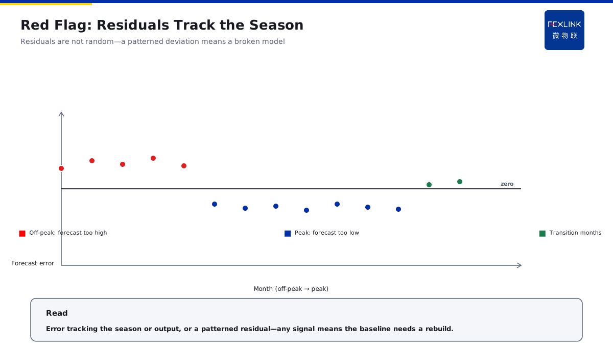
Sign one, peak/off-season jumping — the prediction drifts: the prediction is high in the off-season and low in the peak season; Sign two, concentrated error — the bias clusters: the error clusters around shutdowns and start-stop periods; Sign three, seasonal failure — cross-season inaccuracy: the model clearly fails in another season; Sign four, assessment disputes — each side argues: the peak and off-season data do not match and both sides argue.
In one sentence: the signs of distortion are peak/off-season jumping, concentrated error, cross-season inaccuracy and assessment disputes — identify the four signals first, then diagnose.
The identification signals of distortion — the prediction error is related to season: positive in summer and negative in winter; the error is related to production: the prediction is low in high-production months; the residual plot is regular: the residuals are not random but follow variables — when any signal appears, the baseline needs re-diagnosis.
An example: A factory baseline: one model is forced over the whole year — the off-season prediction is generally 15% high, the peak season is generally 10% low and shutdown months are near zero — both sides argue in the assessment. The logic is that in a company with heavy production fluctuation, the energy structure itself is changing — low load in the off-season, full load in the peak season and near zero in shutdown periods — one model forced over the whole year inevitably fails at both ends — look at the signs of distortion first and then treat the cause.
2. The Effect of Missing Independent Variables (Shifts, Production Schedule, Equipment Status)
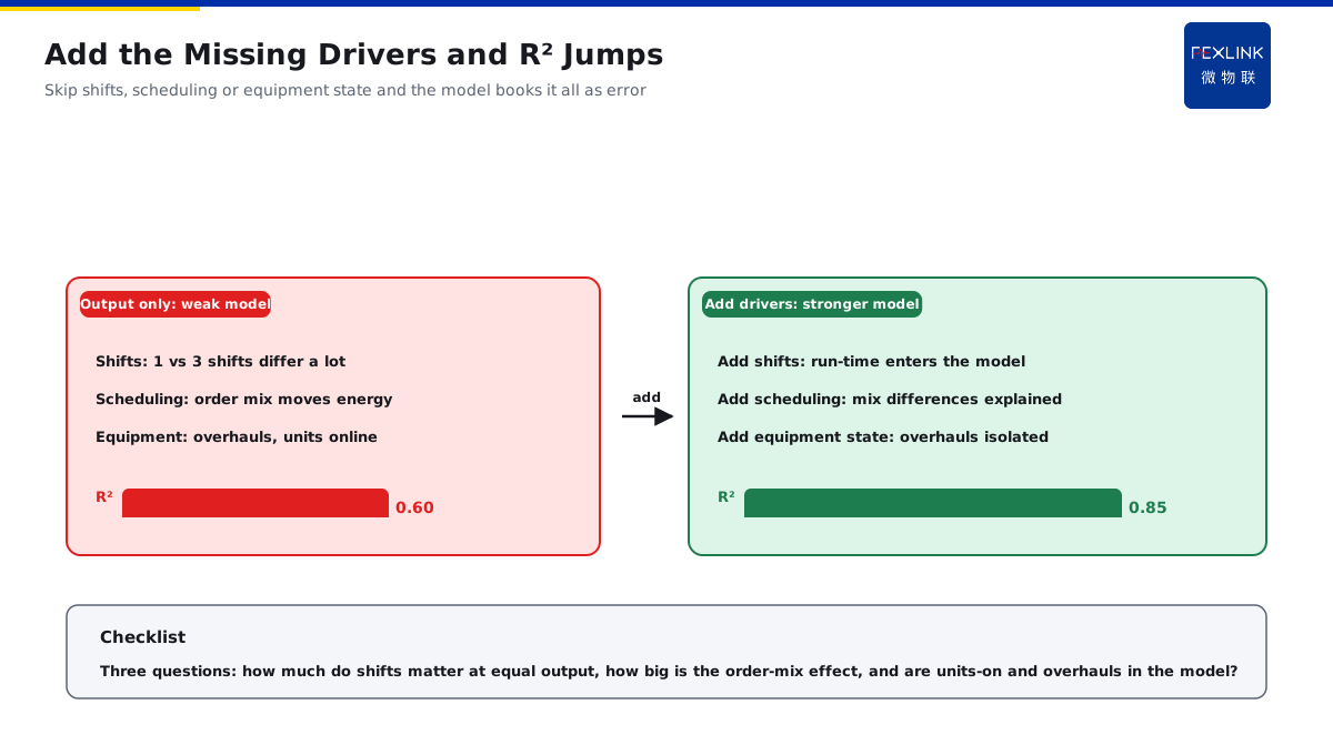
Missing shifts — running hours are not in the model: with the same production, one shift and three shifts differ greatly in energy; Missing the schedule — the production structure is not in the model: different order structures differ greatly in energy; Missing equipment status — start-stop conditions are not in the model: the number of running machines and maintenance status affect energy; Missing others — auxiliary systems are not in the model: auxiliary loads such as air compressors and air conditioning are missed.
In one sentence: missing variables are shifts, the production schedule and equipment status — the model explains less and the prediction drifts — add variables before changing the model.
The check-list of missing variables — ask three questions: how much do different shifts differ in energy at the same production? How much does the order-structure change affect energy? Are the number of running machines and maintenance status in the model? — when any effect is obvious, add the variable.
An example: A factory investigates: the model contains only production — at the same production, three-shift months are clearly higher in energy than one-shift months — after adding the shift variable, R² rises from 0.6 to 0.85, a clear improvement. The logic is that production is not the only driver — shifts, the production schedule and equipment status all affect energy — when variables are missing, the model counts their effects into the error — add the key variables and the explanatory power improves immediately.
3. How to Identify and Remove Abnormal Samples (Shutdowns, Trial Production)
Identification one, shutdown months — abnormally low energy: shutdown and overhaul months do not represent normal production; Identification two, trial-production months — abnormally high energy: trial and commissioning months are high and unstable; Identification three, power-curtailment months — constrained energy: curtailment and peak-shaving months are externally limited; Identification four, event months — disturbed energy: accident and extreme-weather months are abnormal.
In one sentence: abnormal identification is shutdown months, trial-production months, power-curtailment months and event months — mark them, remove them or model them separately — clean samples keep the model stable.
The reference principles of removal — removal is not deletion: mark the reason and archive it for review; removal has a floor: each segment keeps at least 8-10 normal months; re-validate after removal: refit after removal and check whether R² improves clearly.
An example: A factory cleans: from 18 months of data it removes 2 overhaul months and 1 trial-production month — after refitting, R² rises from 0.65 to 0.82. The logic is that abnormal samples are the "pollution source" of the model — overhaul, trial and curtailment months do not represent the normal state — if they stay, the model is pulled aside — identify, mark, remove or handle them separately, and the model is built on the normal production state.
4. Building Segmented Baselines (Peak/Off-Season)
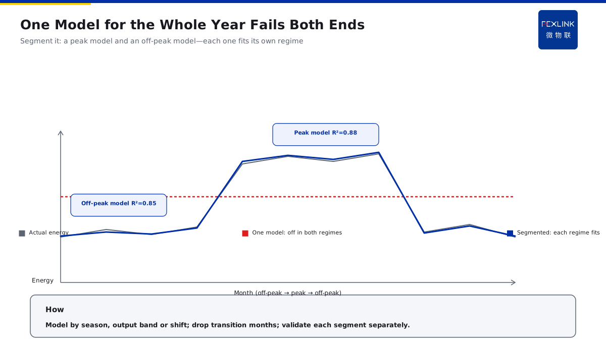
Practice one, model by season — one segment for the peak season and one for the off-season: fit two models separately; Practice two, model by production — a high-production segment and a low-production segment: segment by the production level; Practice three, remove the middle — remove transition months: months between the peak and off-season do not participate; Practice four, boundary validation — validate each segment: check R² and the prediction error of each segment.
In one sentence: the segmented baseline is seasonal/production modeling, transition-month removal and per-segment validation — one model is not forced over the whole year.
The comparison table of segmentation methods:
| Segmentation method | Applicable scenario | Description |
|---|---|---|
| Seasonal modeling | Strong seasonality | One segment for the peak, one for the off-season |
| Production modeling | Wide production range | High-production and low-production segments |
| Shift modeling | Large shift differences | One-shift and three-shift segments |
The implementation steps of segmentation — step one: divide 12-24 months of data by season or production; step two: remove the abnormal samples within each segment; step three: fit a regression model for each segment and check R²; step four: validate the prediction error of each segment and adjust the boundaries when the error is large.
An example: A factory segments: the peak-season model R² is 0.88 and the off-season model R² is 0.85 — both are more accurate than the single whole-year model, a clear difference. The logic is that segmentation is not laziness but respect for the energy structure — the peak season runs full and the off-season runs light, so the energy relationships differ — one model per segment, and every segment is accurate — compared with forcing one model, segmentation fits the actual production better.
5. The Triggers for Periodic Baseline Re-Evaluation
Trigger one, structural change — the production schedule changes: the product structure and the line configuration change greatly; Trigger two, equipment change — new/removed equipment: equipment renewal and capacity change; Trigger three, error out of limit — the prediction error grows: the prediction error keeps exceeding the reasonable range for months; Trigger four, periodic calibration — regular re-evaluation: recommended at least once a year.
In one sentence: the re-evaluation triggers are structural change, equipment change, error out of limit and annual review.
The execution flow of re-evaluation — check the changes first: have the structure and equipment changed greatly? Then look at the error: has the prediction error kept growing over the last three months? Refit: refit the baseline after confirming the trigger; archive and compare: keep the old and new baselines and mark the switch time.
An example: A factory re-evaluates: after adding a new line, the model predicts 8% high for three consecutive months — the re-evaluation is triggered and the model is refit. The logic is that a baseline is alive, not dead — when the production structure and equipment configuration change, the energy relationship changes — the model must follow — a growing error is a signal: re-evaluate first and then use.
Back to the TIANYAN product match — the TIANYAN engine E module (energy analysis) can automatically identify abnormal samples and build segmented models by season or production — for companies with heavy production fluctuation, the system automatically gives a segmented baseline — and automatically prompts re-evaluation when the error grows.
A distorted baseline — first ask two questions: do the variables cover the real operating conditions? Are the samples mixed with abnormal conditions? With heavy production fluctuation, build the baseline in segments and remove the abnormal samples — one model forced over the whole year inevitably fails at both ends — after the diagnosis is clear, the baseline holds and the energy-saving assessment stops being a dispute.
Scope and Limitations
- The conclusions in this article are intended for LV distribution and electrical-safety sites. Criteria are compiled from public codes and FEXLINK product documentation, and product parameters follow the latest selection handbook and product knowledge base.
- Quantitative criteria (protection zone, discharge and residual voltage, earth resistance, thresholds and grading) hold under the preconditions stated in this article. Where the site voltage level, earthing arrangement, environmental category or load profile differs, the figures must be recalculated. Specific configurations involving Tianyan engine, E track (energy analytics) should be verified against actual circuit parameters.
- Specific product models and parameters are subject to the latest selection handbook and product knowledge base; this article does not constitute selection or procurement advice.
- Standard numbers cited here refer to the currently effective editions; when a standard is revised, the related quantitative conclusions must be re-checked.
- Deployment and implementation for specific projects must be carried out by qualified engineers based on site survey and design drawings.
Frequently Asked Questions
With Fluctuating Output and Seasonal Production, Why Does the Calculated Baseline Fall Apart?
With fluctuating output and seasonal production, why does the calculated baseline fall apart