 FEXLINK Research Institute
The short answer
When bills climb back after an efficiency retrofit, the equipment is rarely the problem. Three things are usually missing: savings were never normalized for operating conditions, the money was never calculated against the actual tariff structure, and nobody kept a monthly loop running afterwards. A retrofit answers one question — can this site save energy at all. The loop answers a different one — does the saving stay on the books. The test is simple: is there a metric that runs every month and explains how much less energy this month used against the baseline, and why. Without that, efficiency remains a one-off event rather than an operating capability.
1. Two numbers, not one
Energy savings are physical: kilowatt-hours. Cost savings are financial: currency. Between them sits a tariff sheet, and that sheet turns the same kilowatt-hour into very different amounts of money.
A kilowatt-hour shifted out of the off-peak band might be worth 0.38; the same kilowatt-hour removed from the on-peak band might be worth 1.20. The ratio is roughly three to one. Demand charges make it worse: they are levied on maximum demand or transformer capacity, so a site that cuts consumption without cutting its peak still pays the full demand component. This is how a report claiming "18% energy savings" coexists with a finance team looking at a 4% bill reduction. Nobody miscalculated. Two different ledgers were being kept.
Keep both ledgers: kilowatt-hours for technical verification, currency for payback. A project with only one of them cannot be defended in a review meeting.
2. Why baselines drift
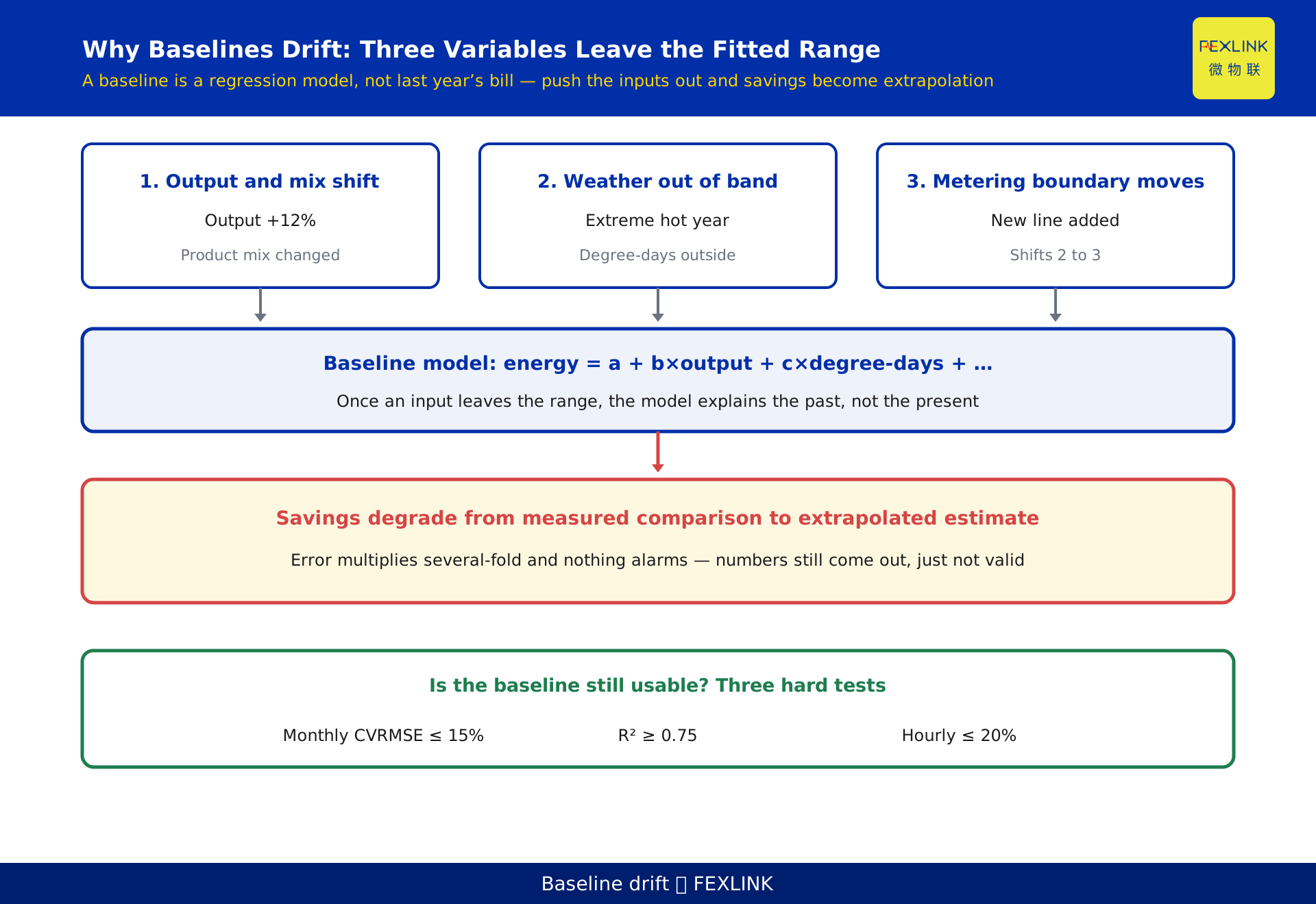
Savings are baseline minus actual. The baseline is not last year's bill; it is a regression model — a constant term, a production coefficient times output, a degree-day coefficient times degree-days, plus whatever else drives load. Get the model right and the difference is real. Get it wrong and the difference is arithmetic.
Three variables make it drift.
Output and product mix move. The model was fitted over a 12-month output range. If output rises 12%, or the plant shifts from low-value to high-value product, the independent variable leaves the fitted range. What comes out is an extrapolation, and extrapolation amplifies error several times over.
Weather leaves the historical band. Cooling and heating loads are strongly degree-day sensitive. Assess an extreme summer against a baseline built on a mild year and the savings appear from nowhere — or vanish.
The metering boundary moves. A new line, an extension, a shift pattern going from two to three. The denominator is no longer the same denominator, and comparing across it is comparing two different things.
There is a hard test for whether a baseline still holds: for monthly models, CVRMSE no greater than 15% and R-squared no lower than 0.75, per ASHRAE Guideline 14; hourly models relax to 20%. Beyond that line the model cannot be used to compute savings — it has to be rebuilt.
3. Four pockets on the bill
An industrial bill is not one number. It is four components added together, and savings may land in only one of them.
| Component | Charged on | Can efficiency reduce it |
|---|---|---|
| Energy charge | Time-of-use kilowatt-hours times band rate | Yes, but on-peak and off-peak differ roughly threefold |
| Demand charge | Transformer capacity or maximum demand | Only if the peak falls; consumption cuts do nothing |
| Power factor adjustment | Power factor, 0.90 standard | New VFDs and rectifiers lower it, so the charge can rise |
| Government funds and surcharges | Per kilowatt-hour | Falls proportionally with consumption |
The first two are where the money is. Cut consumption without cutting the peak and the demand component stays at full price. Add variable frequency drives without reactive compensation and power factor slides from 0.93 to 0.88, so the power factor adjustment eats part of the gain.
4. A worked example: 1.1 million promised, 252,000 delivered
The following is an illustrative scenario, constructed to show how the arithmetic diverges. It does not represent any specific customer or project.
A campus with two 10 kV incomers and two 1250 kVA transformers. Baseline year: output 1.0 million units, consumption 8.60 million kWh, annual bill 6.20 million, specific consumption 8.60 kWh per unit. The retrofit covered compressor waste-heat recovery, LED lighting, and VFDs on fans and pumps, at a cost of 1.80 million.
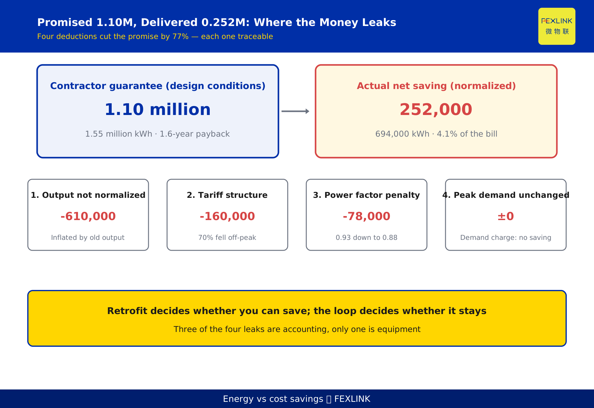
The contractor, working from design conditions, guaranteed 1.55 million kWh and 1.10 million in annual savings, with a 1.6-year payback.
In the first year after retrofit, output rose to 1.12 million units and consumption reached 8.94 million kWh. Specific consumption fell to 7.98 kWh per unit — 7.2% below baseline. Normalized, real savings are 0.62 times 1.12 million, or 694,000 kWh: 45% of the guarantee.
Now the money. About seventy percent of those 694,000 kWh fell in the off-peak band, at a weighted 0.475 per kWh, worth roughly 330,000. The new VFDs had no compensation, so power factor dropped from 0.93 to 0.88 and the power factor adjustment added 78,000. Peak demand did not fall, so the demand charge saved nothing. Net saving: 252,000, or 4.1% of the original bill.
What the owner saw: the bill moved from 6.20 million to 6.45 million — up 4%. "We spent 1.8 million and the bill went up" is exactly how that sentence gets said.
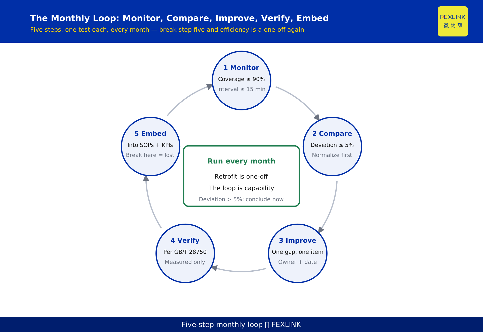
5. The monthly loop: monitor, compare, improve, verify, embed
The difference between a one-off retrofit and continuous improvement is whether a loop actually runs every month.
Monitor. Data completeness comes first. A main meter shows the total; sub-meters show where. Target: at least 90% coverage of major load circuits, intervals no coarser than 15 minutes.
Compare. Set the month's EnPI against the baseline, compute the deviation, and normalize for conditions. A deviation beyond plus or minus 5% needs a conclusion this month, not at year end.
Improve. Once the deviation is traced to a circuit, open a work item: one deviation, one item, with owner, budget and date.
Verify. Measure per GB/T 28750 after completion. Do not back-calculate from nameplate efficiency times running hours.
Embed. Write what worked into operating procedures, into crew performance measures, into the asset register. Skip this and the next shift supervisor will dial the parameters back.
Step five is where loops break. The first four speak project language; the fifth speaks management language. Crossing that line is what makes it a loop.
Step two depends on the energy performance indicator, or EnPI. One is never enough, though more is not automatically better.
Production looks at specific consumption, kWh per unit. Offices and commercial space look at energy per square metre. Management looks at energy per unit of revenue. Three indicators, three levels — mix them and they contradict each other. When output drops, specific consumption can rise while energy per unit revenue falls. Which one you put in the scorecard decides the conclusion.
The test for a good EnPI is correlation: it should explain more than 70% of consumption variance. An indicator that cannot do that only generates arguments.
6. Three ways verification goes wrong
Re-baselining after the retrofit. The most common self-certifying move: take post-retrofit data as the new baseline and every month afterwards shows savings. The baseline must be locked before the work starts, versioned, with every change logged.
Substituting theory for measurement. Nameplate efficiency times running hours assumes the equipment runs at full load at design conditions. Real load factors sit at 40% to 60%, so the theoretical figure overstates savings by more than double.
Skipping normalization. Comparing twelve months after against twelve months before, with output, weather and boundary unadjusted, is both the largest error and the most common practice.
One more point that gets overlooked: metering accuracy has to match the size of the saving. Verifying a 5% saving with a class 1 meter means the meter's own error is close to 1% — the signal-to-noise ratio is too low for the conclusion to stand. Measurement and verification metering should be class 0.5S or better.
7. Preventing rebound
Rebound is rarely an equipment problem. It is an incentive problem. Savings accrue to the company; the crew that produced them feels nothing. Parameters drift back to where they were comfortable, predictably.
Three moves hold it down.
First, push EnPIs down to crew level, publish rankings monthly, tie them to performance. The indicator must be at a granularity the crew can influence: total bill is beyond them, one line's specific consumption is not.
Second, automate exception tickets. When daily consumption deviates more than 8% from baseline, generate a ticket to the shift supervisor with a 48-hour close requirement. Same-day handling is the cheapest handling.
Third, re-baseline only when the boundary genuinely changes. Re-baselining an unchanged boundary hands back savings already earned.
8. Where products fit
A loop runs on data, and data starts at the endpoint.
Circuit-level metering with the ESA all-element smart meter (for example ESA-22131-R, 3×400A, 3×220/380V, RS485 Modbus) — one per circuit, read per shift — answers "which line caused the deviation." Where phase and harmonic data are needed, the ESB three-phase imbalance monitor or the ESE series applies.
Above that, the Tianyan engine (the forecasting layer, 67 predictive models) does two jobs: normalize the month's consumption against output and degree-days, and forecast next month's baseline band so deviation raises an alarm early instead of surfacing in the monthly report.
At the top, the energy performance improvement framework ties it together, mapping to the energy baseline, EnPI and performance improvement triad in ISO 50001 and GB/T 23331. Sites that also manage carbon can connect the 4×3×2 energy-carbon autonomy framework so energy and emissions report on one set of definitions.
9. Three things handover usually drops
Loops break at handover more often than at commissioning.
The equipment manual is handed over; the baseline file is not. The model, the list of independent variables, CVRMSE and R-squared, the historical data window used to fit — this is the foundation for every future savings calculation. Without it, the successor starts from zero, and the pre-retrofit data is gone.
Metering points and ratios go unchecked. A meter installed on the main incomer but analysed as if it were a circuit-level point, or a current transformer ratio that does not match the meter setting. Readings can be off by a factor of two or five, and nothing alarms — the error quietly bends every conclusion downstream. Verify ratio, phase sequence and connection group on site, and keep a record.
The contract never defines how savings are calculated. "Guaranteed 18% savings" without specifying baseline construction, normalization method, metering class or verifier leaves both sides free to disagree at acceptance. That is the most expensive blank in an energy performance contract.
10. FAQ
The bill went up after the retrofit. Does that mean it failed?
Not necessarily. Higher output and added equipment raise the bill on their own. The test is specific energy: did it fall, and by how much. In the example, the bill rose 4% while specific consumption fell 7.2% — the retrofit worked, but the savings claim was inflated and the cost calculation was wrong.
Who should calculate the savings?
Someone who does not carry the retrofit target. A contractor grading its own savings is a candidate marking its own exam. A third party or the site's energy management function should apply GB/T 28750, with the baseline locked before work begins and changes logged.
Can we run the loop without sub-meters?
You can detect problems but not locate them. Start by metering the circuits that account for more than 70% of consumption; there is no need to cover the whole plant at once.
How often should the baseline be rebuilt?
Only when the boundary changes: new line, extension, shift pattern change, major process change. Rebuilding an unchanged baseline erases savings already realized.
Does ISO 50001 certification mean the loop is in place?
No. Certification examines management system documentation and review records. The loop is about whether monthly data actually runs. Plenty of certified sites still have no monthly EnPI tracking.
Scope and limitations
- The savings and cost algorithms discussed here apply to high-voltage commercial and industrial users on two-part tariffs. Single-part tariff users can omit the demand charge analysis.
- The CVRMSE 15% and R-squared 0.75 thresholds are quoted from ASHRAE Guideline 14 as methodology. Project contracts may set their own model acceptance thresholds, but should not go below these.
- Data in the worked example is constructed to illustrate the arithmetic, is labelled an illustrative scenario, and does not represent any real customer or project. Actual investment, savings and payback require site survey and measured data.
- The 0.90 power factor standard follows the current power factor adjustment rules; local implementation details and assessment bands vary, and the local utility's interpretation governs.
- Model numbers and specifications for the ESA all-element smart meter, the ESB three-phase imbalance monitor and the Tianyan engine are subject to the latest selection manual and product knowledge base. This article is not a selection or procurement recommendation.
- Standard numbers cited are current as of writing; if a standard is revised, the quantitative conclusions here require rechecking.
Frequently Asked Questions
Why Do Bills Climb Back After an Efficiency Retrofit
When bills climb back after an efficiency retrofit, the equipment is rarely the problem