 微物联研究院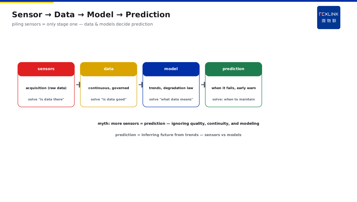
Direct Answer
Enterprises think that installing more sensors enables predictive maintenance, yet end up with piles of data but no predictions? The answer: the key to predictive maintenance is not the number of sensors, but whether the degradation process can be described by continuous data and whether a degradation model is available; without historical data accumulation and trend modeling, more sensors only provide real-time display; first select the key degradation quantities, accumulate data, then talk about prediction — this is the core of correcting the misconception.
One plant installed 200 sensors at once (vibration/temperature/current full coverage), assuming "more data means predictions." Six months later, faults were still found by on-site inspection; the data platform was only a "real-time display" tool. Review: no historical data accumulation (the normal-to-fault process data was missing), no degradation model (no idea which trend foretells a fault) — more sensors meant "seeing" without "understanding." Rectification: first select 5 key degradation quantities (bearing temperature, vibration severity, current trend, etc.), accumulate a 6-month baseline continuously, then build a degradation-trend model. Prediction core: continuous data describing degradation + an available degradation model — sensors are the acquisition means, not the prediction itself.
Because:
- More sensors ≠ prediction: data is the raw material; the model is the prediction;
- Two prerequisites are both indispensable: continuous data describing degradation + an available degradation model;
- Historical data is the "training set": without the complete normal→fault process, no trend can be built;
- Real-time display ≠ prediction: seeing the current value is not knowing when it will fail.
Key insight: "select degradation quantities, accumulate data, build the model" — these three steps are predictive maintenance. Hardware piling is only the first step — data quality and models determine prediction capability.
One group launched a "plant-wide sensors" project (500 points) with millions invested; a year later, fault-prediction success was under 10% and auditors questioned it. Review: sensor types were mixed (no priority), data unwashed (noisy), no degradation model (only real-time curves). Lesson: piling hardware produces no prediction — "select + accumulate + model" is indispensable; verify on a small scope first, then roll out.
1. Why More Sensors ≠ Prediction
Step one: why piling sensors does not work.
The role of sensors:
- Sensors = acquisition means (data raw material);
- Data = input (raw material fed to the model);
- Model = prediction capability (finding patterns in data);
- The chain: sensor → data → model → prediction.
Misconceptions of piling sensors:
- Quantity thinking: assuming "more = better";
- Ignoring data quality: noisy/unstable sampling, inconsistent definitions;
- Ignoring data continuity: occasional sampling cannot describe the degradation process;
- Ignoring model building: data without a model = real-time display only.
The essence of prediction:
- Prediction = inferring the future from trends (degradation modeling);
- Needs: continuous data (process) + degradation model (pattern);
- Sensors only solve "is there data";
- The model solves "what the data means."
Key insight: "sensors + data + model" is the three-stage structure of predictive maintenance. Only piling sensors means only the first stage — data and models determine prediction capability.
2. The Two Prerequisites for Prediction
Step two: what conditions enable prediction.
Prerequisite one: the degradation process can be described by continuous data:
- Key degradation quantities: temperature/vibration/current/partial discharge, etc. (select well);
- Continuous acquisition: minute-level/hour-level (process visible);
- Data quality: stable sampling, accurate calibration, no gaps;
- Degradation features: trend/rate/abrupt change (identifiable signals).
Prerequisite two: an available degradation model:
- Historical data: the complete normal→abnormal→fault process;
- Trend modeling: threshold/rate/statistical models;
- Model verification: verify prediction accuracy with historical data;
- Continuous updating: the model iterates as data accumulates.
Both prerequisites are indispensable:
- Data without model: real-time display only;
- Model without data: the model has nothing to work on;
- Both present: degradation describable, faults predictable.
Key insight: "continuous data describing degradation + an available degradation model" are the two hard prerequisites. Missing either, prediction is only a slogan.
3. The Importance of Data Accumulation
Step three: why data must be accumulated first.
The value of data:
- Historical data = the "video" of the degradation process;
- Normal baseline: the data pattern when equipment is healthy;
- Degradation process: the trajectory from normal to fault;
- Model training: build prediction patterns from historical data.
Accumulation points:
- Select the right degradation quantities: quantities related to the fault mechanism (not greedy);
- Continuous acquisition: no interruption (complete process);
- Data annotation: record maintenance/fault events (correspondence);
- Quality governance: de-noising, cleaning, calibration (model reliability).
Accumulation cycles:
- Baseline building: weeks to months (normal pattern);
- Complete process: ideally including one maintenance/fault cycle;
- Continuous accumulation: the longer the better (model iteration);
- Accumulate while verifying: simple thresholds first, then trend models.
Key insight: "data accumulation" is the foundation of predictive maintenance. Select the right degradation quantities + continuous acquisition + quality governance — the model has a "training set."
4. Common Features of Failed Cases
Step four: why many projects fail.
Common feature one: hardware thinking:
- Sensor count as a KPI;
- Point coverage as achievement;
- Data quality and models ignored.
Common feature two: data gaps:
- Discontinuous acquisition (gapped sampling);
- Unwashed data (noise pollution);
- No event annotation (unknown correspondence).
Common feature three: missing model:
- Real-time curves only (no trend analysis);
- Threshold alarms only (no degradation prediction);
- No model verification (accuracy unknown).
Common feature four: rushing:
- Demanding predictions immediately after go-live (no data accumulation);
- Rolling out at once (no small-scope verification);
- No ROI evaluation (cannot quantify).
Key insight: failed projects ≈ "hardware + display" projects, missing the "data + model" links. Self-check against the four features — avoid the same pitfalls.
5. Correct Implementation Sequence
Step five: how to proceed step by step.
Correct sequence:
- Step 1: select key degradation quantities (3–10, related to the fault mechanism);
- Step 2: accumulate data (weeks to months, including the normal baseline);
- Step 3: build the model (thresholds first, then trends, iterating);
- Step 4: verify on a small scope (1–2 machines validate predictions);
- Step 5: roll out and optimize (expand after verification; model continuously updated).
Implementation points:
- Small first, then large: verify before rollout (risk control);
- Data first: guarantee data quality before model building;
- Business alignment: prediction results linked to maintenance plans;
- Continuous iteration: the model keeps optimizing as data accumulates.
Effect evaluation:
- Prediction accuracy: share of faults hit;
- Lead time: how early the warning comes (maintenance window);
- Missed-alarm rate: share of unpredicted faults;
- ROI: reduced unplanned downtime and maintenance costs.
Key insight: "select → accumulate → model → verify → roll out" is the correct path. Make it work on a small scope first, then expand — avoid "plant-wide sensors" investment failures.
6. Product Landing: Predictive Maintenance Solution
FEXLINK products land predictive maintenance:
- Key-degradation-quantity monitoring: temperature/vibration/partial discharge/current, etc. (select first, then install);
- Data-platform accumulation: historical data and trend analysis;
- Degradation models: combined threshold + trend + rate judgment;
- Prediction reports: early warnings linked to maintenance recommendations.
Design principle in one sentence: "select degradation quantities, accumulate data, build the model." No quantity piling, results first — predictive maintenance truly lands.
7. Common Misconception Checklist
- More sensors = prediction: mistaking acquisition for prediction. Consequence: piles of data, no predictions. Correct: model building first.
- Real-time display = prediction: claiming prediction because you can see the current value. Consequence: fault found only when it happens. Correct: trend modeling.
- Predicting immediately at go-live: without data accumulation. Consequence: the model has nothing to work on. Correct: accumulate baseline first, then model.
- Plant-wide rollout at once: promoting without verification. Consequence: problems amplified, investment wasted. Correct: verify on a small scope, then roll out.
- Data without governance: modeling on noisy data directly. Consequence: inaccurate model, many misjudgments. Correct: clean and calibrate data first.
Scope and Limitations
This article clarifies the misconception "predictive maintenance = more sensors" and provides a correct implementation framework for predictive maintenance (two prerequisites, data accumulation, correct sequence), applicable to predictive-maintenance planning and project evaluation for electrical equipment. Specific degradation-quantity selection must follow equipment type and fault mechanism; model building requires a certain period (data accumulation and verification); prediction-effect evaluation criteria must follow on-site maintenance practices. All cases are anonymized (a certain plant/a certain group) and do not refer to any specific customer.