 微物联研究院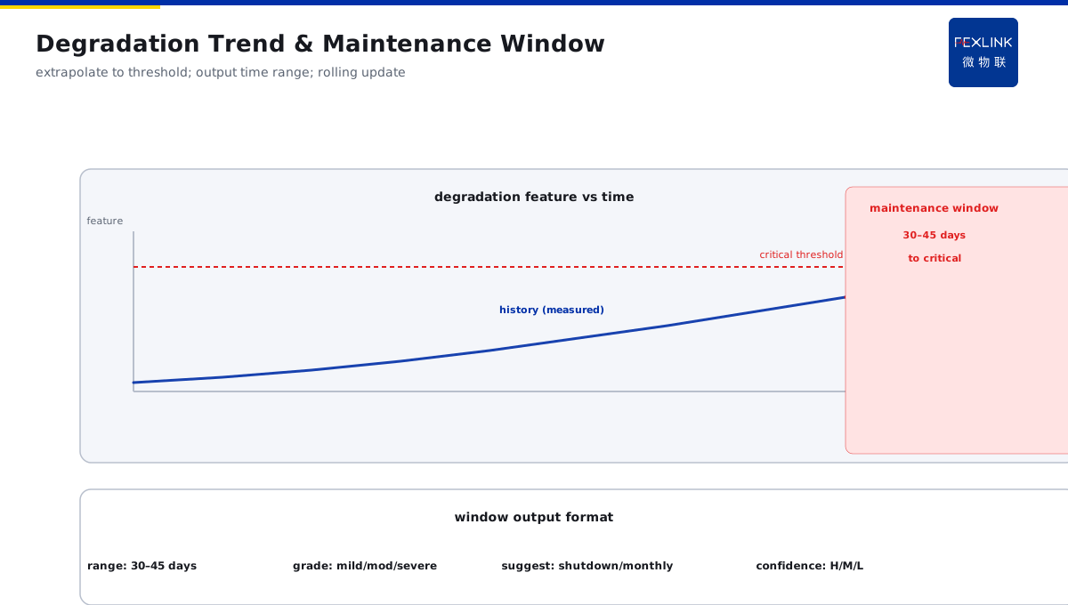
Direct Answer
How should a predictive-maintenance scheme be designed for the power supply circuits of critical production lines? The answer: close the loop in five steps — sensing-point configuration, feature extraction, degradation prediction, maintenance window, production coordination. Place temperature, current, leakage, and PD sensing points on critical circuits; extract features at the edge; predict degradation trends on the platform and output an "estimated degradation window"; maintenance is then scheduled within that window instead of at fixed intervals. The value of the scheme lies in "turning unplanned downtime into planned maintenance."
At an auto-parts plant, the critical production line (running 24/7; one hour of downtime costs ¥200,000) had its power circuits maintained on a fixed half-year cycle. After adopting predictive maintenance: circuits got temperature, current, and leakage points; the platform output an "estimated degradation window" per circuit (e.g., "contact-resistance degradation, expected to reach critical in 30–45 days"). In the third month, one panel's contact-resistance trend went abnormal; the platform gave a 20-day window, the plant arranged maintenance inside the National Day shutdown window, and replaced the risky joint in advance — avoiding unplanned downtime. The core loop of a predictive-maintenance scheme is: sensing → features → trend → window → maintenance, turning "fixed-cycle" into "window-based scheduling."
Because:
- Sensing points decide "whether a degradation signal exists": temperature (contact/overload), current (load trend), leakage (insulation degradation), PD (insulation defects) — four point types cover the main degradation modes;
- Feature extraction decides "whether degradation is visible": raw data ≠ degradation trend; features such as baseline deviation, slope, and fluctuation must be extracted;
- Prediction outputs a "window," not a "number": a time range gives maintenance schedulable lead time;
- The maintenance window must link to the production plan: pick an outage/low-load slot inside the window — this is where predictive maintenance delivers value.
Key insight: predictive maintenance is a closed loop from sensing points to maintenance, not "installing sensors and watching curves." Once the five-step loop runs, unplanned downtime becomes planned maintenance.
At a cement plant, a critical circuit's busbar temperature trend went abnormal; the platform predicted "likely critical within 30 days," and the plant handled it inside the planned maintenance window (replacing the busbar joint). By handling time, the measured temperature was already near threshold — under the fixed cycle (still 3 months away), unplanned downtime would have occurred. The window prediction gave operators lead time, turning emergency repair into calm planning.
1. Sensing-Point Configuration on Critical Circuits
Step one: how to configure points. Four point types cover the main degradation modes:
Temperature points (contact/overload degradation):
- Positions: busbar joints, breaker contacts, cable joints, transformer windings;
- Role: early signal of increased contact resistance and overload;
- Reference: joint-vs-adjacent ΔT (watch at ΔT ≥ 5 °C);
- Quantity: 3–6 temperature points per circuit (per equipment structure).
Current points (load trend):
- Positions: circuit incomer, branch feeders;
- Role: load trend, three-phase unbalance, overload risk;
- Reference: load-factor trend (watch at load factor ≥ 80%);
- Quantity: 1–2 per circuit (incomer + key branch).
Leakage points (insulation degradation):
- Positions: circuit leakage monitoring (residual current);
- Role: insulation aging, moisture, precursor of insulation breakdown;
- Reference: residual-current trend (steady → slowly rising = insulation degradation);
- Quantity: 1 per circuit (leakage-monitoring module).
PD points (insulation defects):
- Positions: switchgear, transformers (critical equipment);
- Role: partial discharge in insulation (early defect signal);
- Reference: PD trend (growing with load = real defect);
- Quantity: 1–2 per critical equipment (TEV/UHF).
Configuration principles:
- Critical circuits (large downtime loss): full configuration (temperature + current + leakage + PD);
- General circuits: basic monitoring (temperature + current);
- Standardized point numbering, matching the ledger;
- Cost grading: high configuration on critical, basic on general.
Key insight: point configuration is the sensing foundation. Temperature, current, leakage, PD — four types cover the main degradation modes; configure fully on critical circuits first.
2. Degradation-Trend Modeling Inputs
Step two: how the degradation trend is computed. Feature extraction is the prediction input:
Feature extraction:
- Baseline deviation: current value vs historical baseline (deviation magnitude);
- Slope: rate of trend rise/fall (steeper = faster degradation);
- Fluctuation: short-term variation (large fluctuation = unstable);
- Correlation: correlation with load (distinguishes real degradation vs load change).
Modeling inputs:
- Historical data: at least 3–6 months of continuous data (baseline establishment);
- Event records: maintenance, replacement, alarm records (model calibration);
- Operating conditions: load, ambient temperature (removes interference factors);
- Feature set: baseline deviation + slope + fluctuation + correlation (into the model).
Model methods:
- Simple and reliable: trend extrapolation (linear/exponential fitting);
- Advanced: degradation-curve fitting (bathtub curve, exponential degradation);
- Higher: machine learning (needs abundant historical data; use with care);
- Principle: simple and reliable first, then advanced — do not complicate for its own sake.
Modeling principles:
- Data quality first: reject bad data (dropouts, interference);
- Interpretability: the model output must be explainable (why this window);
- Continuous calibration: new data enters; the model updates periodically;
- Conservative principle: leave margin in the predicted window (early rather than late).
Key insight: feature extraction is the key to "whether degradation is visible." Baseline deviation + slope + fluctuation + correlation — four features feed the model, and only then is the degradation trend predictable.
3. Maintenance-Window Output Format
Step three: how prediction results are output. A window beats a number:
Window output format:
- "Expected to reach critical in 30–45 days" (a time range, not a point);
- "Current degradation level: mild / moderate / severe" (state grading);
- "Suggested window: National Day shutdown / monthly maintenance / weekend low load" (production-coordination advice);
- "Confidence: high / medium / low" (reliability labeling).
How the window is computed:
- Extrapolation: extrapolate the current slope to the threshold (simple and direct);
- Grading: degradation level maps to disposition deadline (mild = continue monitoring; moderate = planned maintenance; severe = handle immediately);
- Rolling update: prediction refreshed daily (window corrected as data rolls);
- Threshold setting: per OEM advice + historical experience (e.g., 90 °C critical temperature).
Value of the window:
- Gives operators lead time (not "what now" but "when");
- Gives production plan-ability (window can meet shutdown plans);
- Gives management a decision basis (cost–benefit computable);
- Gives maintenance optimization space (schedule within window, no emergency repair).
Window examples:
- Contact-resistance degradation: ΔT-trend extrapolation, critical in 30–45 days;
- Insulation degradation: slowly rising leakage, 60–90 days;
- PD defect: grows with load, alarm level in 2–4 weeks.
Key insight: the maintenance window is executable output. Time range + state grade + production-coordination advice + confidence — operators can schedule on receipt; production can plan on receipt.
4. Coordination with the Production Plan
Step four: how a window becomes maintenance. Coordination is the key:
Coordination flow:
- Platform outputs the maintenance window (estimated degradation time range);
- Operations reviews the production plan (shutdown windows, low-load slots);
- Selects the nearest suitable slot inside the window (schedule within lead time);
- Arranges maintenance (work order → spares → manpower → execute in the window);
- Re-measures after maintenance (confirm degradation removed, trend fallen back).
Coordination principles:
- Lead time first: the earlier the window, the more room to choose;
- Minimal production impact: prefer shutdown windows / low-load slots;
- Spares ready: spares in place within the window (no delay);
- Multi-party alignment: production, operations, and maintenance align the time.
Coordination scenarios:
- Planned shutdown window (annual maintenance / holidays): merge directly when the window matches;
- Monthly maintenance window: moderate degradation merges into the monthly plan;
- Emergency window: severe degradation coordinates a temporary shutdown (less loss than unplanned downtime);
- Rolling window: re-evaluate as the window nears (upgrade handling if lead time is insufficient).
Coordination benefits:
- Unplanned downtime → planned maintenance (loss drops sharply);
- Higher maintenance-resource utilization (no emergency repair);
- Production-plan certainty (know in advance when a stop is needed).
Key insight: coordination with the production plan is where value is realized. Window → plan → maintenance → re-measure; done well, predictive maintenance actually lands.
5. Scheme-Effectiveness Metrics
Step five: how effectiveness is measured. Metrics must be quantifiable:
Core metrics:
- Unplanned-downtime count (target: 50%+ reduction);
- Maintenance timeliness (share completed within the window);
- Prediction hit rate (window prediction vs actual degradation time);
- False-alarm rate (share of alarms confirmed as non-defect; target < 20%).
Process metrics:
- Point online rate (data completeness);
- Feature-extraction coverage (all features on critical circuits);
- Window-output rate (share of critical circuits with a window prediction);
- Maintenance-loop closure rate (alarm–work order–maintenance–re-measure fully closed).
Value metrics:
- Downtime-loss reduction (quantified in money);
- Maintenance-cost optimization (planned vs emergency-repair cost);
- Equipment-life extension (early handling slows degradation);
- ROI (investment vs downtime-loss reduction).
Measurement approach:
- Pre-launch baseline (existing downtime data);
- Continuous post-launch statistics (monthly/quarterly comparison);
- Key-circuit focused tracking (high-value circuits listed separately);
- Platform auto-reports (metrics automatically tallied).
Rollout cadence:
- Weeks 1–2: point installation, commissioning, ledger setup;
- Weeks 3–8: data accumulation, baseline establishment, feature-extraction tuning;
- Weeks 9–12: prediction model launch, window-output validation;
- From week 13: rolling operation, metric statistics, model calibration;
- Two phases: phase 1 critical circuits (2–3 high-value), phase 2 expansion to all critical circuits.
Key insight: effectiveness metrics make the scheme verifiable. Fewer unplanned stops, window hits, maintenance-loop closure — metrics speak; cost–benefit is computable.
6. Product Landing: Predictive-Maintenance Scheme
FEXLINK products bring the predictive-maintenance scheme to the field:
- ESX Edge Computing Gateway: sensing-point aggregation, feature extraction, local trend pre-judgment;
- EST Multi-Channel Temperature Controller: multi-point temperature on circuits, ΔT trend (contact-degradation signal);
- Electrical Fire Monitor / Leakage Monitoring: residual-current trend (insulation-degradation signal);
- PD monitoring: PD trend on critical equipment (insulation-defect signal);
- The platform outputs an "estimated degradation window" plus maintenance advice, with work-order linkage closed loop.
Design principle in one sentence: upgrade "fixed-cycle maintenance" into "window-based scheduling." Sensing → features → trend → window → maintenance, a five-step loop — unplanned downtime becomes planned maintenance.
7. Common Scheme-Design Mistakes
- Only temperature, nothing else: missing current/leakage/PD. Consequence: degradation modes not fully covered. Correct: four point types configured per critical circuit.
- Data without features: collect but never extract. Consequence: raw data shows no degradation trend. Correct: extract baseline deviation + slope + fluctuation + correlation.
- Predicting a number, not a window: only "X days left." Consequence: a single-point prediction is unreliable; operators hesitate. Correct: output a time range + confidence.
- Window not linked to production: prediction without scheduling. Consequence: prediction wasted; maintenance still reactive. Correct: link the window to shutdown/low-load slots.
- No effectiveness measurement: ignoring metrics after launch. Consequence: effect unprovable; investment not sustained. Correct: continuously track unplanned stops, hit rate, etc.
Scope and Limitations
This article provides an overall framework for a predictive-maintenance scheme on critical-load power circuits (point configuration, feature extraction, window output, production coordination, effectiveness metrics) for predictive-maintenance project design on critical production lines / important supply circuits. Point configuration and cost grading should be adjusted to circuit importance and budget; prediction models primarily use trend extrapolation and grading; machine learning needs sufficient historical data; the maintenance window is a predictive reference and requires manual confirmation against on-site conditions; outage maintenance must follow procedures by qualified personnel. Online monitoring data is managed uniformly through the platform to form trend alerts. All cases are anonymized (an auto-parts plant / a cement plant) and do not refer to any specific customer.